Next: 3.4 FastReplica in the
Up: 3 FastReplica Algorithm
Previous: 3.2 FastReplica in the
3.3 Preliminary Performance Analysis of FastReplica in the Small
Let  denote the transfer time of file
  from the original
node
from the original
node  to node
  as measured at node . We use
transfer time and replication time interchangeably in the text.
In our study, we consider the following two performance metrics:
as measured at node . We use
transfer time and replication time interchangeably in the text.
In our study, we consider the following two performance metrics:
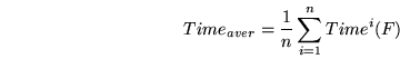
- Average replication time:
- Maximum replication time:
 reflects the time when all the nodes in the replication
set receive a copy of the original file, and the primary goal of
FastReplica is to minimize the maximum replication time. However, we
are also interested in understanding the impact of FastReplica
on the average replication time
reflects the time when all the nodes in the replication
set receive a copy of the original file, and the primary goal of
FastReplica is to minimize the maximum replication time. However, we
are also interested in understanding the impact of FastReplica
on the average replication time  .
First, let us consider an idealistic setting, where nodes
.
First, let us consider an idealistic setting, where nodes
 have symmetrical (or nearly symmetrical) incoming and
outgoing bandwidth which is typical for CDNs, distributed IDCs, and a
distributed enterprise environment. In addition, let nodes
have symmetrical (or nearly symmetrical) incoming and
outgoing bandwidth which is typical for CDNs, distributed IDCs, and a
distributed enterprise environment. In addition, let nodes
 be homogeneous, and let each node can support
  network
connections to other nodes at
network
connections to other nodes at  bytes per second on average.
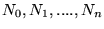
Figure 4:
Uniform-random
model: speedup in file replication time under FastReplica vs Multiple Unicast for a different number of nodes
in replication set for a) average replication time, and b) maximum
replication time.
 |
In the idealistic setting, there is no difference between maximum and
average replication times. Using the assumption on homogeneity of nodes'
bandwidth, we can estimate the transfer time for each concurrent
connection 
 during the distribution step:
 |
(1) |
The transfer time at the collection step is similar to the time encountered at the first (distribution) step:
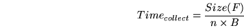 |
(2) |
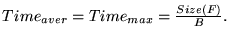
Thus the overall replication time under FastReplica in the small
is the following:
 |
(3) |
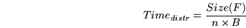
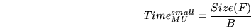
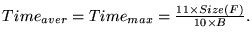
Let Multiple Unicast denote a schema that transfers the entire
file from the original node to nodes
 by
simultaneously using
by
simultaneously using  concurrent network connections. The overall
transfer time under Multiple Unicast is the following:
concurrent network connections. The overall
transfer time under Multiple Unicast is the following:
 |
(4) |
Thus, in an idealistic setting, FastReplica in the small provides the
following speedup of file replication time compared to the
Multiple Unicast strategy:
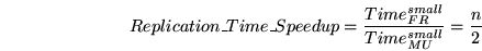 |
(5) |
While the comparison of FastReplica and Multiple Unicast
in the idealistic environment gives insights into why the new
algorithm may provide significant performance benefits for replication
of the large files, the bandwidth conditions in the realistic setting
could be very different from the idealistic assumptions. Due to
changing network conditions, even the same link might have a different
available bandwidth when measured at different times.
Let us analyze how FastReplica performs when network paths
participating in the transfers have a different available bandwidth.
Let  denote a bandwidth matrix, where
 ![$BW[i][j]$](img50.png) reflects
the available bandwidth of the path from node to node
reflects
the available bandwidth of the path from node to node  as measured at some time
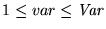
  , and let Var be
the ratio of maximum to minimum available bandwidth along the paths
participating in the file transfers. We call Var a
bandwidth variation.
In our analysis, we consider the bandwidth matrix to be populated in
the following way:
, and let Var be
the ratio of maximum to minimum available bandwidth along the paths
participating in the file transfers. We call Var a
bandwidth variation.
In our analysis, we consider the bandwidth matrix to be populated in
the following way:
where function
 returns a random integer
  :
:
 .
While it is still a simplistic model, it helps to reflect a realistic
situation, where the available bandwidth of different links can be
significantly different. We will call this model a uniform-random model.
To perform a sensitivity analysis of how the FastReplica
performance depends on a bandwidth variation of participating paths, we
experimented with a range of different values for Var between
.
While it is still a simplistic model, it helps to reflect a realistic
situation, where the available bandwidth of different links can be
significantly different. We will call this model a uniform-random model.
To perform a sensitivity analysis of how the FastReplica
performance depends on a bandwidth variation of participating paths, we
experimented with a range of different values for Var between
 and
and  . When
  , it is the idealistic setting,
discussed above, where all of the paths are homogeneous and have the
same bandwidth (i.e. no variation in bandwidth). When
, it is the idealistic setting,
discussed above, where all of the paths are homogeneous and have the
same bandwidth (i.e. no variation in bandwidth). When
 , the network paths between the nodes have highly variable
available bandwidth with a possible difference of up to 10 times.
Using the uniform-random model and its bandwidth matrix , we
compute the average and maximum file replication times under
FastReplica and Multiple Unicast methods for a different number
of nodes in the replication set, and derive the relative speedup of
the file replication time under FastReplica compared to the
replication time under the Multiple Unicast strategy. For each
value of Var, we repeated the experiments multiple times, where
the bandwidth matrix is populated by using the random number
generator with different seeds.
Figure 4 a) shows the relative average replication
time speedup under FastReplica in the small compared to
Multiple Unicast in the uniform-random model. For Var=2,
the average replication time for 8 nodes under FastReplica
is 3 times better compared to Multiple Unicast, and for
20 nodes, it is 8 times better. While the performance
benefits of FastReplica against Multiple Unicast are
decreasing for higher variation of bandwidth of participating paths,
FastReplica still remains quite efficient, with performance
benefits converging to a practically fixed ratio for
, the network paths between the nodes have highly variable
available bandwidth with a possible difference of up to 10 times.
Using the uniform-random model and its bandwidth matrix , we
compute the average and maximum file replication times under
FastReplica and Multiple Unicast methods for a different number
of nodes in the replication set, and derive the relative speedup of
the file replication time under FastReplica compared to the
replication time under the Multiple Unicast strategy. For each
value of Var, we repeated the experiments multiple times, where
the bandwidth matrix is populated by using the random number
generator with different seeds.
Figure 4 a) shows the relative average replication
time speedup under FastReplica in the small compared to
Multiple Unicast in the uniform-random model. For Var=2,
the average replication time for 8 nodes under FastReplica
is 3 times better compared to Multiple Unicast, and for
20 nodes, it is 8 times better. While the performance
benefits of FastReplica against Multiple Unicast are
decreasing for higher variation of bandwidth of participating paths,
FastReplica still remains quite efficient, with performance
benefits converging to a practically fixed ratio for  .
Figure 4 b) shows the relative maximum replication
time speedup under FastReplica in the small compared to
Multiple Unicast in the uniform-random model. We can observe
that, independent of the values of bandwidth variation, the maximum
replication time under FastReplica for n nodes is
.
Figure 4 b) shows the relative maximum replication
time speedup under FastReplica in the small compared to
Multiple Unicast in the uniform-random model. We can observe
that, independent of the values of bandwidth variation, the maximum
replication time under FastReplica for n nodes is  times better compared to the maximum replication time under
Multiple Unicast.
It can be explained in the following way:
times better compared to the maximum replication time under
Multiple Unicast.
It can be explained in the following way:
 Multiple Unicast:
The maximum replication time is
defined by the entire file transfer time over the path with the worst
available bandwidth among the paths connecting and ,
Multiple Unicast:
The maximum replication time is
defined by the entire file transfer time over the path with the worst
available bandwidth among the paths connecting and ,
 .
.
FastReplica:
Figure 5 shows the set of paths participating in
the file transfer from node to node  under the
FastReplica algorithm (we use as a representative of the recipient nodes).
under the
FastReplica algorithm (we use as a representative of the recipient nodes).
Figure 5:
FastReplica in the small: a set of paths used in file replication from node to node .
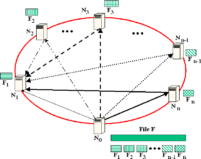 |
The replication time observed at node is defined by the maximum
transfer time of  -th of the file over either:
- the path from to , or
- the path with the worst overall available bandwidth consisting of
two subpaths:
- the subpath from to and
- the subpath from to ,
for some
 .
.
In the considered uniform-random model, a worst case
scenario is when both subpaths have a minimal bandwidth, and since
each path is used for transferring -th of the entire file,
this would lead to times latency improvement under
FastReplica compared to the maximum replication time under
Multiple Unicast.
Now, let us consider a special, somewhat artificial example, which
aims to provide an additional insight into the possible performance
outcomes under FastReplica when the values of bandwidth matrix
are significantly skewed.
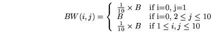
Let be the origin node, and
 be the recipient
nodes, and the bandwidth between the nodes be defined by the following
matrix:
be the recipient
nodes, and the bandwidth between the nodes be defined by the following
matrix:
 |
(6) |
In other words, the origin node has a limited bandwidth of
 to node , while the bandwidth from
to the rest of the recipient nodes
to node , while the bandwidth from
to the rest of the recipient nodes
 is equal to . In
addition, the cross-bandwidth between the nodes
is
also very limited, such that any pair and is connected via
a path with available bandwidth of
.
At a glance, it seems that FastReplica might perform badly in
this configuration because the additional cross-bandwidth between the
recipient nodes
is so poor relative to the bandwidth
available between the origin node and the recipient nodes
. Let us compute the average and maximum replication
times for this configuration under Multiple Unicast and
FastReplica strategies.
is equal to . In
addition, the cross-bandwidth between the nodes
is
also very limited, such that any pair and is connected via
a path with available bandwidth of
.
At a glance, it seems that FastReplica might perform badly in
this configuration because the additional cross-bandwidth between the
recipient nodes
is so poor relative to the bandwidth
available between the origin node and the recipient nodes
. Let us compute the average and maximum replication
times for this configuration under Multiple Unicast and
FastReplica strategies.
Multiple Unicast:
FastReplica:
The maximum replication time in this configuration is  times better
under FastReplica than under Multiple Unicast. In
FastReplica, any path between the nodes is used to transfer only
-th of the entire file. Thus, the paths with poor bandwidth
are used for much shorter transfers which leads to a significant
improvement in maximum replication time. However, the average
replication time in this example is not improved under
FastReplica compared to Multiple Unicast. The reason for this
is that the high bandwidth paths in this configuration are used
similarly: to transfer only -th of the entire file, and
during the collection step of the FastReplica algorithm, the
transfers of complementary -th size subfiles within the
replication group are performed over poor bandwidth paths. Thus, in
certain cases, like considered above, FastReplica may provide
significant improvements in maximum replication time, but may not
improve the average replication time.
The analysis considered in this section outlines the conditions when
FastReplica is expected to perform well, providing the essential
performance benefits. Similar reasoning can be applied to derive the
situations when FastReplica might be inefficient. For example,
let us slightly modify the previous example. Let the bandwidth matrix
be defined in the following way:
times better
under FastReplica than under Multiple Unicast. In
FastReplica, any path between the nodes is used to transfer only
-th of the entire file. Thus, the paths with poor bandwidth
are used for much shorter transfers which leads to a significant
improvement in maximum replication time. However, the average
replication time in this example is not improved under
FastReplica compared to Multiple Unicast. The reason for this
is that the high bandwidth paths in this configuration are used
similarly: to transfer only -th of the entire file, and
during the collection step of the FastReplica algorithm, the
transfers of complementary -th size subfiles within the
replication group are performed over poor bandwidth paths. Thus, in
certain cases, like considered above, FastReplica may provide
significant improvements in maximum replication time, but may not
improve the average replication time.
The analysis considered in this section outlines the conditions when
FastReplica is expected to perform well, providing the essential
performance benefits. Similar reasoning can be applied to derive the
situations when FastReplica might be inefficient. For example,
let us slightly modify the previous example. Let the bandwidth matrix
be defined in the following way:
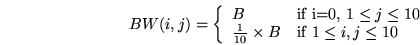 |
(7) |
In this configuration, the bandwidth from the origin node
to the rest of the recipient nodes
is equal to , while
the cross-bandwidth between the nodes
is
very limited: any pair and is connected via
a path with available bandwidth of
.
The average and maximum replication
times for this configuration under Multiple Unicast and
FastReplica strategies can be computed as follows:
Multiple Unicast:
FastReplica:
Thus in this configuration, FastReplica does not
provide any performance benefits.
In a general case, if there is a node  in the replication set
such that most of the paths between and the rest of the nodes
have a very limited available bandwidth (say, times worse than the
minimal available bandwidth of the paths connecting and ,
) then the performance of FastReplica during the
second (collection) step is impacted by the poor bandwidth of the
paths between and ,
in the replication set
such that most of the paths between and the rest of the nodes
have a very limited available bandwidth (say, times worse than the
minimal available bandwidth of the paths connecting and ,
) then the performance of FastReplica during the
second (collection) step is impacted by the poor bandwidth of the
paths between and ,
 and FastReplica
will not provide expected performance benefits. Note, that (the
number of nodes in the replication group) plays a very important role
here: a larger value of provides a higher ``safety'' level for
FastReplica efficiency. A larger value of helps to offset a
higher difference in bandwidth between the available bandwidth within the
replication group and the available bandwidth from the original node
to the nodes in the replication group.
To apply FastReplica efficiently, the preliminary bandwidth
estimates are useful. These bandwidth estimates are also essential for
correct clustering of the appropriate nodes into the replication
subgroups in FastReplica in the large discussed in the next
section.
and FastReplica
will not provide expected performance benefits. Note, that (the
number of nodes in the replication group) plays a very important role
here: a larger value of provides a higher ``safety'' level for
FastReplica efficiency. A larger value of helps to offset a
higher difference in bandwidth between the available bandwidth within the
replication group and the available bandwidth from the original node
to the nodes in the replication group.
To apply FastReplica efficiently, the preliminary bandwidth
estimates are useful. These bandwidth estimates are also essential for
correct clustering of the appropriate nodes into the replication
subgroups in FastReplica in the large discussed in the next
section.
Next: 3.4 FastReplica in the
Up: 3 FastReplica Algorithm
Previous: 3.2 FastReplica in the