Amdahl's Law & Parallel Speedup

The theory of doing computational work in parallel has some fundamental laws that place limits on the benefits one can derive from parallelizing a computation (or really, any kind of work). To understand these laws, we have to first define the objective. In general, the goal in large scale computation is to get as much work done as possible in the shortest possible time within our budget. We ``win'' when we can do a big job in less time or a bigger job in the same time and not go broke doing so. The ``power'' of a computational system might thus be usefully defined to be the amount of computational work that can be done divided by the time it takes to do it, and we generally wish to optimize power per unit cost, or cost-benefit.

Physics and economics conspire to limit the raw power of individual single processor systems available to do any particular piece of work even when the dollar budget is effectively unlimited. The cost-benefit scaling of increasingly powerful single processor systems is generally nonlinear and very poor - one that is twice as fast might cost four times as much, yielding only half the cost-benefit, per dollar, of a cheaper but slower system. One way to increase the power of a computational system (for problems of the appropriate sort) past the economically feasible single processor limit is to apply more than one computational engine to the problem.

This is the motivation for beowulf design and construction; in many cases a beowulf may provide access to computational power that is available in a alternative single or multiple processor designs, but only at a far greater cost.

In a perfect world, a computational job that is split up among $N$ processors would complete in $1/N$ time, leading to an $N$-fold increase in power. However, any given piece of parallelized work to be done will contain parts of the work that must be done serially, one task after another, by a single processor. This part does not run any faster on a parallel collection of processors (and might even run more slowly). Only the part that can be parallelized runs as much as $N$-fold faster.

The ``speedup'' of a parallel program is defined to be the ratio of the rate at which work is done (the power) when a job is run on $N$ processors to the rate at which it is done by just one. To simplify the discussion, we will now consider the ``computational work'' to be accomplished to be an arbitrary task (generally speaking, the particular problem of greatest interest to the reader). We can then define the speedup (increase in power as a function of $N$) in terms of the time required to complete this particular fixed piece of work on 1 to $N$ processors.

Let $T(N)$ be the time required to complete the task on $N$ processors. The speedup $S(N)$ is the ratio

$$S(N) = \frac{T(1)}{T(N)}.$$ (1)

In many cases the time $T(1)$ has, as noted above, both a serial portion $T_s$ and a parallelizeable portion $T_p$. The serial time does not diminish when the parallel part is split up. If one is "optimally" fortunate, the parallel time is decreased by a factor of $1/N$). The speedup one can expect is thus

$$S(N) = \frac{T(1)}{T(N)} = \frac{T_s + T_p}{T_s + T_p/N}.$$ (2)

This elegant expression is known as Amdahl's Law [Amdahl] and is usually expressed as an inequality. This is in almost all cases the best speedup one can achieve by doing work in parallel, so the real speed up $S(N)$ is less than or equal to this quantity.

Amdahl's Law immediately eliminates many, many tasks from consideration for parallelization. If the serial fraction of the code is not much smaller than the part that could be parallelized (if we rewrote it and were fortunate in being able to split it up among nodes to complete in less time than it otherwise would), we simply won't see much speedup no matter how many nodes or how fast our communications. Even so, Amdahl's law is still far too optimistic. It ignores the overhead incurred due to parallelizing the code. We must generalize it.

A fairer (and more detailed) description of parallel speedup includes at least two more times of interest:

${\bf T_s}$ The original single-processor serial time.

${\bf T_{is}}$ The (average) additional serial time spent doing things like interprocessor communications (IPCs), setup, and so forth in all parallelized tasks. This time can depend on $N$ in a variety of ways, but the simplest assumption is that each system has to expend this much time, one after the other, so that the total additional serial time is for example $N*T_{is}$.

${\bf T_p}$ The original single-processor parallelizeable time.

${\bf T_{ip}}$ The (average) additional time spent by each processor doing just the setup and work that it does in parallel. This may well include idle time, which is often important enough to be accounted for separately.

It is worth remarking that generally, the most important element that contributes to $T_{is}$ is the time required for communication between the parallel subtasks. This communication time is always there - even in the simplest parallel models where identical jobs are farmed out and run in parallel on a cluster of networked computers, the remote jobs must be begun and controlled with messages passed over the network. In more complex jobs, partial results developed on each CPU may have to be sent to all other CPUs in the beowulf for the calculation to proceed, which can be very costly in scaled time. As we'll see below, $T_{is}$ in particular plays an extremely important role in determining the speedup scaling of a given calculation. For this (excellent!) reason many beowulf designers and programmers are obsessed with communications hardware and algorithms.

It is common to combine $T_{ip}$, $N$ and $T_{is}$ into a single expression $T_o(N)$ (the ``overhead time'') which includes any complicated $N$-scaling of the IPC, setup, idle, and other times associated with the overhead of running the calculation in parallel, as well as the scaling of these quantities with respect to the ``size'' of the task being accomplished. The description above (which we retain as it illustrates the generic form of the relevant scalings) is still a simplified description of the times - real life parallel tasks can be much more complicated, although in many cases the description above is adequate.

Using these definitions and doing a bit of algebra, it is easy to show that an improved (but still simple) estimate for the parallel speedup resulting from splitting a particular job up between $N$ nodes (assuming one processor per node) is:

$$S(N) = \frac{T_s + T_p}{T_s + N*T_{is} + T_p/N + T_{ip}}.$$ (3)

This expression will suffice to get at least a general feel for the scaling properties of a task that might be parallelized on a typical beowulf.

Figure 1: $T_{is} = 0$ and $T_p =$ 10, 100, 1000, 10000, 100000 (in increasing order).

It is useful to plot the dimensionless ``real-world speedup'' (3) for various relative values of the times. In all the figures below, $T_s$ = 10 (which sets our basic scale, if you like) and $T_p$ = 10, 100, 1000, 10000, 100000 (to show the systematic effects of parallelizing more and more work compared to $T_s$).

The primary determinant of beowulf scaling performance is the amount of (serial) work that must be done to set up jobs on the nodes and then in communications between the nodes, the time that is represented as $T_{is}$. All figures have $T_{ip} = 1$ fixed; this parameter is rather boring as it effectively adds to $T_s$ and is often very small.

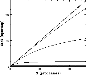
Figure 1 shows the kind of scaling one sees when communication times are negligible compared to computation. This set of curves is roughly what one expects from Amdahl's Law alone, which was derived with no consideration of IPC overhead. Note that the dashed line in all figures is perfectly linear speedup, which is never obtained over the entire range of $N$ although one can often come close for small $N$ or large enough $T_p$.

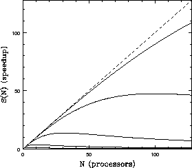
In figure 2, we show a fairly typical curve for a ``real'' beowulf, with a relatively small IPC overhead of $T_{is} = 1$. In this figure one can see the advantage of cranking up the parallel fraction ($T_p$ relative to $T_s$) and can also see how even a relatively small serial communications process on each node causes the gain curves to peak well short of the saturation predicted by Amdahl's Law in the first figure. Adding processors past this point costs one speedup. Increasing $T_{is}$ further (relative to everything else) causes the speedup curves to peak earlier and at smaller values.

Finally, in figure 3 we continue to set $T_{is} = 1$, but this time with a quadratic $N$ dependence $N^2*T_{is}$ of the serial IPC time. This might result if the communications required between processors is long range (so every processor must speak to every other processor) and is not efficiently managed by a suitable algorithm. There are other ways to get nonlinear dependences of the additional serial time on $N$, and as this figure clearly shows they can have a profound effect on the per-processor scaling of the speedup.

Figure 2: $T_{is} = 10$ and $T_p =$ 10, 100, 1000, 10000, 100000 (in increasing order).

Figure 3: $T_{is} = 10$ and $T_p =$ 10, 100, 1000, 10000, 100000 (in increasing order) with $T_{is}$ contributing quadratically in $N$.

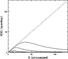As one can clearly see, unless the ratio of $T_p$ to $T_{is}$ is in the ballpark of 100,000 to 1 one cannot actually benefit from having 128 processors in a ``typical'' beowulf. At only 10,000 to 1, the speedup saturates at around 100 processors and then decreases. When the ratio is even smaller, the speedup peaks with only a handful of nodes working on the problem. From this we learn some important lessons. The most important one is that for many problems simply adding processors to a beowulf design won't provide any additional speedup and could even slow a calculation down unless one also scales up the problem (increasing the $T_p$ to $T_{is}$ ratio) as well.

The scaling of a given calculation has a significant impact on beowulf engineering. Because of overhead, speedup is not a matter of just adding the speed of however many nodes one applies to a given problem. For some problems it is clearly advantageous to trade off the number of nodes one purchases (for example in a problem with small $T_s$ and $T_p/T_{is} \approx 100$) in order to purchase tenfold improved communications (and perhaps alter the $T_p/T_{is}$ ratio to 1000).

The nonlinearities prevent one from developing any simple rules of thumb in beowulf design. There are times when one obtains the greatest benefit by selecting the fastest possible processors and network (which reduce both $T_s$ and $T_p$ in absolute terms) instead of buying more nodes because we know that the rate equation above will limit the parallel speedup we might ever hope to get even with the fastest nodes. Paradoxically, there are other times that we can do better (get better speedup scaling, at any rate) by buying slower processors (when we are network bound, for example), as this can also increase $T_p/T_{is}$. In general, one should be aware of the peaks that occur at the various scales and not naively distribute small calculations (with small $T_p/T_{is}$) over more processors than they can use.

In summary, parallel performance depends primarily on certain relatively simple parameters like $T_s$, $T_p$ and $T_{is}$ (although there may well be a devil in the details that we've passed over). These parameters, in turn are at least partially under our control in the form of programming decisions and hardware design decisions. Unfortunately, they depend on many microscopic measures of system and network performance that are inaccessible to many potential beowulf designers and users. $T_p$ clearly should depend on the ``speed'' of a node, but the single node speed itself may depend nonlinearly on the speed of the processor, the size and structure of the caches, the operating system, and more.

Because of the nonlinear complexity, there is no way to a priori estimate expected performance on the basis of any simple measure. There is still considerable benefit to be derived from having in hand a set of quantitative measures of ``microscopic'' system performance and gradually coming to understand how one's program depends on the potential bottlenecks they reveal. The remainder of this paper is dedicated to reviewing the results of applying a suite of microbenchmark tools to a pair of nodes to provide a quantitative basis for further beowulf hardware and software engineering.