
Because the real processors on which we implemented RightSpeed derive little efficiency from using one setting versus another, PACE cannot save sufficient energy on them to make its implementation worthwhile. To evaluate the effectiveness of our PACE calculator, in this section we conduct simulations assuming future processors with better DVS characteristics. Our simulations differ from those in [11] since we do not make the same assumptions about scheduling capabilities. In particular, we consider a finite number of settings and limited timer granularity.
For our simulations, we consider three processors, each with a minimum setting running at 200 MHz and consuming 1 W, and each with power consumption proportional to speed cubed. (This cubic relationship assumes either a very low threshold voltage or a threshold voltage that is varied proportionally to supply voltage using technology like that in [8].) The three processors differ only in their maximum speeds: 600 MHz, 800 MHz, and 1 GHz. We assume the processors can only run at multiples of 50 MHz and the timer granularity is 0.1 ms.
Since our simulations occur on virtual hardware, we can run them much faster than real time. So, we can use longer workloads than those in Table 4, which were restricted to a single application. Instead, we use eight workloads, each corresponding to all activity of a traced user.
All the algorithms we simulate, except for the no-DVS algorithm, will use the same performance target, so that we can compare them fairly using only energy consumption. The performance target is to have an average pre-deadline speed of 400 MHz and a post-deadline speed of 600 MHz. The four algorithms we consider are:
| ||||||||||||||||||||||||||||||||||||||||||||||||||||||||||||||||||||||||||||||||||||||||||||||||||||||||||||||||||||||||||||||||||||
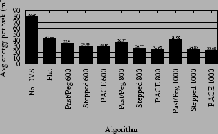 |
One interesting observation is that the greater the range of speeds available on the CPU, the more energy efficient the Stepped and PACE algorithms become. For example, per-task average CPU energy consumption under PACE decreases 19.5% when switching from a CPU with maximum speed 600 MHz to one with maximum speed 1 GHz. This is because the availability of a higher speed on the CPU allows a schedule to begin a task running more slowly, since it can more easily make up for this slowness by running even faster later in the schedule. The ability to run slowly at the beginning saves energy in the common case where the task requires little work, since the schedule never proceeds past the low-energy beginning part. PACE takes advantage of the broader range of speeds to find a better schedule, while Stepped just happens to work better with the larger set of speeds. Past/Peg, on the other hand, does worse with a greater range of speeds. Essentially, Past/Peg ignores all but the two extreme settings of the CPU, and we see that this is costly in terms of energy consumption; we conclude that using intermediate speeds can save energy.
We also see from these results that PACE is always the best algorithm, followed by Stepped, followed by Past/Peg, followed by Flat. This echoes the results from [12], and shows that even when we require PACE to deal with limited settings and timer granularity, it is still an improvement over existing DVS algorithms.
Furthermore, we predicted in Section 3 that the greater the available CPU speed range, the better PACE would do in comparison to other algorithms, and we see this borne out in our simulation results. On the CPU with maximum speed 600 MHz, PACE reduces energy consumption by 6.1% compared to Stepped; with maximum speed 800 MHz, the reduction is 8.0%; with maximum speed 1 GHz, the reduction is 8.7%.
In conclusion, we find that even when a finite set of speeds are available and the timer granularity is limited, PACE is still an improvement over other algorithms. We find that having higher speeds available on the CPU helps PACE reduce energy consumption, and furthermore PACE does better the greater the range of speeds available on the CPU. This is an important lesson for chip designers, who may think that providing the capability of running at high voltages and therefore high speeds will increase energy consumption. We see here that with proper energy management using PACE, provision of higher speeds can actually reduce energy consumption.