|
NSDI '05 Paper
[NSDI '05 Technical Program]


IP Fault Localization Via Risk Modeling
Ramana Rao Kompella2, Jennifer Yates3,
Albert Greenberg3, Alex C. Snoeren2
2 University of California, San Diego, {ramana,snoeren}@cs.ucsd.edu
3 AT&T Labs - Research,
{jyates,albert}@research.att.com
Abstract:
Automated, rapid, and effective fault management is a central goal of
large operational IP networks. Today's networks suffer from a wide
and volatile set of failure modes, where the underlying fault proves
difficult to detect and localize, thereby delaying repair. One of the
main challenges stems from operational reality: IP routing and the
underlying optical fiber plant are typically described by disparate
data models and housed in distinct network management systems.
We introduce a fault-localization methodology based on the use of risk
models and an associated troubleshooting system, SCORE (Spatial
Correlation Engine), which automatically identifies likely root causes
across layers. In particular, we apply SCORE to the problem of localizing link
failures in IP and optical networks. In experiments conducted on
a tier-1 ISP backbone, SCORE proved remarkably effective at localizing
optical link failures using only IP-layer event logs.
Moreover,
SCORE was often able to automatically uncover inconsistencies in the
databases that maintain the critical associations between the IP and optical
networks.
1 Introduction
Operational IP networks are intrinsically exposed to a wide variety of faults
and impairments. These networks are large, geographically distributed,
constantly evolving, with complex hardware and software artifacts. A typical
tier-1 network consists of about 1,000 routers from different vendors, with
different features, and acting in different roles in the network architecture.
Such a network is supported by access and core transport networks, which
typically involve at least two orders of magnitude more network elements
(optical amplifiers, Dense Wavelength Division Multiplexing (DWDM) systems,
ATM/MPLS/Ethernet switches, and so forth). These network elements and
associated telemetry generate a large number of management events relating to
performance and potential failure conditions. The essential problem of IP fault
management is to monitor the event stream to detect, localize, mitigate and
ultimately correct any condition that degrades network behavior.
Unfortunately, operational IP networks today lack intrinsic robustness; serious
faults and outages are not infrequent. While existing fault management systems
(e.g., [12,21,8]) provide great value in automating
routine fault management, serious problems can fly ``under the radar,'' or, once
detected, cannot be rapidly localized and diagnosed. To appreciate why this is
so, it may help to imagine a network operator faced with the task of IP fault
management.
After much effort, network hardware has been designed and implemented, the
protocols controlling the network have been designed (often in compliance with
published standards), and the associated software implemented. In accord with
the network architecture, the network elements have been deployed, connected,
and configured. Yet, all these complex endeavors are carried out by multiple
teams at rapid pace, involving a large and distributed software component, thus
producing operational artifacts far richer in behavior than can ever be
approximated in a lab. Errors will be introduced at each stage of network
definition and go undetected despite best practices in design, implementation,
and testing. External factors, including bugs of all types (memory leaks,
inadequate performance separation between processes, etc.) in router software
and environmental factors such as DoS attacks and BGP-related traffic events
originating in peer networks significantly raise the level of difficulty. It is
the task of IP fault management to cope with the result, continually learning
and dealing with new failure modes in the field.
In this paper, we introduce a risk modeling methodology that allows for faster,
more accurate automatic localization of IP faults to support both real-time and
offline analysis. By design, we:

- split our solution into generic algorithmic components
(Section 4.2) and problem domain specific components (Section 4.5), and
-
- create risk models that reflect fundamental architectural elements of
the problem domain, but not necessarily implementation details.
As a result, our system is robust
to churn in operational networks and is more likely to be extensible
to additional system components.
We apply our methodology to the specific problem of fault localization across IP
and optical network layers, a difficult problem faced by network operators
today. Currently, when IP operations receives router-interface alarms, the
systems and staff are often faced with time-intensive manual investigation of
what layer the problem occurred in, where, and why. This task is hampered by
the architecture of the underlying network: IP uses optics for transport and (in
some cases) for self-healing services (e.g., SONET ring restoration) in an
overlay fashion. The task of managing each of the two network layers is
naturally separated into independent software systems.
Joining dynamic fault data across IP and optical systems is
highly challenging--the network elements, supporting standards and
information models are totally different. Though there are fields,
such as circuit IDs, which can be used to join databases across these
systems, automated mechanisms to assure the accuracy of these joins
are lacking. Unfortunately, the network elements and protocols
provide little help. Path-trace capabilities (counterparts of IP
traceroute) are not available in the optical layer, or, if available,
do not work in a multi-vendor environment (e.g., where the DWDM
systems are provided by multiple vendors). In optical systems such as
SONET, there is no counterpart to IP utilization statistics, which
might be used to correlate traffic at the IP layer with the optical
layer. Both IP and optical network topologies are rapidly changing as
equipment is upgraded, network reach is extended, and capacities are re-engineered to manage changing demands.
Our key contribution is the novel and successful application of risk modeling to
localize faults across the IP and optical layers in operational networks.
Roughly speaking, a physical object such as a fiber span or an optical amplifier
represents a shared risk for a group of logical entities (such as IP
links) at the IP layer. That is, if the optical device fails or degrades, all
of the IP components that had relied upon that object fail or degrade. In the
literature, these associations are referred to as Shared Risk Link Groups
or SRLGs [4]. Using only event data gathered at IP layer, and
topology data gathered at both IP and optical layers, we bridge the gap between
the operational information network managers need and what is actually reported
at IP layer. SCORE (Spatial Correlation Engine) relieves operators of the
burden of cross-correlating dynamic fault information from two disparate network
layers. Once the layer and the location of the fault has been determined, other
systems and tools at the appropriate layer can be targeted towards identifying
the precise characteristics (for example, rule-based or statistical
methods [12,21]).
2 Troubleshooting using shared risks
Monitoring alarms associated with IP network component failures are
typically generated on an individual basis--for example, a router
failure will appear as a failure of all of the links terminating at
that router. Best current practice requires a manual correlation of
the individual link failure notifications to determine that they are
all a result of a common network element (e.g., router).
In more complicated failure scenarios, however,
it is substantially more challenging to group individual alarms
into common groups, and often difficult to even identify in
which layer the fault occurred (e.g., in the transport network
interconnecting routers, or in the routers themselves).
By identifying the set of possible components that could have caused
the observed symptoms, shared risk analysis can serve as the first
step of diagnosing a network problem. For events being investigating by
operations personnel in real time, reducing the time required
for troubleshooting directly decreases down time.
Our challenge is to construct a model of risks that represent the set
of IP links that would likely be impacted by the failure of each
component within the network. The tremendous complexity of the
hardware and software upon which an IP network is built implies that
constructing a model that accounts for every possible failure mode
is impractical. Instead, we identify the key components of the risk model
that represent the prevalent network failure modes and those that do
not require deep knowledge of each vendor's equipment used within
the network. We hasten to add that the better the SRLG modeling of
the network, the more precise the fault diagnosis can be. However, as
we show later, a solid SRLG model combined with a flexible spatial
correlation algorithm can ensure that fault isolation can be robust to
missing details in the risk model developed.
Figure 1:
Example illustrating the concept of SRLGs.
|
The basic network topology can be represented as a set of nodes
interconnected via links. Inter-domain and intra-domain routing protocols such
as OSPF and BGP operate with a basic abstraction of a point-to-point link
between a routers. Of course, OSPF permits other abstractions such as
multi-access and non-broadcast, but a backbone network typically only consists
of point-to-point links between routers. Figure 1 illustrates a very
simplistic network consisting of five nodes connected via six optical links
(circuits). Each inter-office IP link is carried on an optical circuit
(typically using SONET). This optical circuit in turns consists of a series of
one or more fibers, optical amplifiers, SONET rings, intelligent optical mesh
networks and/or DWDM systems [18]. These systems consist of
network elements that provide O-E-O (optical to electrical) conversion and, in
the case of SONET rings or mesh optical networks, protection/restoration to
recover from optical layer failures. Multiple optical fibers are then carried in
a single conduit, commonly known as a fiber span. Typically, each optical
component may carry multiple IP links--the failure of these components would
result in the failure of all of these IP links. We illustrate this concept in
the bottom half of Figure 1, where we show the optical layer topology
over which the IP links are routed. In the Figure 1, these shared risks
are denoted as FIBER SPAN 1 to 6, DWDM 1 and 2. CKT3 and CKT5 are both routed
over FIBER SPAN 4 and thus would both fail with the failure of FIBER SPAN 4.
Similarly DWDM 1 is shared between CKT 1, 3, 4 and 5, while CKT 6 and CKT 7
share DWDM 2.
In essence, each network element represents a shared risk among all
the links that traverse through this element. Hence, this set of links
represents what is known as the Shared Risk Link Group (SRLG), as
defined in
[14,23]. This concept is well understood in the context
of network planning where backup paths are chosen such that they do
not have any SRLG in common with the primary path, and sufficient
capacity is planned to survive SRLG failures. However, the application
of risk group models to real-time and offline fault analysis has not
been well explored.
We now present the shared risk group model that we construct to
represent a typical IP network. We divide the model into
hardware-related risks and software risks. Note that this model is
not exhaustive, and can be expanded to incorporate, for example,
additional software protocols.
Fiber: At the lowest level, a single optical fiber carries multiple
wavelengths using DWDM. One
or more IP links are carried on a given wavelength. All wavelengths
that propagate through a fiber form an SRLG with the fiber being the
risk element. A single fiber cut can simultaneously induce faults on
all of the IP links that ride over that fiber.
Fiber span: In practice, a set of fibers are carried together
through a cable. A set of cables are laid out in a conduit. A cut
(from, e.g., a backhoe) can simultaneously fail all links carried
through the conduit. These set of circuits that ride through the
conduit form the fiber span SRLG.
SONET network elements: In practice SONET network elements such as optical
amplifiers, add-drop multiplexors etc., are shared across multiple wavelengths
(that represent the circuits). For example, an optical amplifier amplifies all
the wavelengths simultaneously - hence a problem in the optical amplifier can
potentially disrupt all associated wavelengths. We collectively group these
elements together into the SONET network elements group.
Router modules: A router is usually composed of a set of
modules, each of which can terminate one or more IP links. A
module-related SRLG denotes all of the IP links terminating on the
given module, as these would all be subject to failure should the
module die.
Router: A router typically terminates a significant number of IP
links, all of which would likely be impacted by a router failure
(either software or hardware). Hence, all of the IP links
terminating on a given router collectively belong to a given router
SRLG.
Ports: An individual link can also fail due to the failure of a single
port on the router (impacting only the one link), or through other failure modes
that impact only the single link. Thus, we also include Port SRLGs in our model.
Port SRLGs however are singleton sets consisting of only one circuit. However,
we add them in our risk model in order to be able to explain single link
failure.
Autonomous system: An autonomous system (AS)
is a logical grouping of routers within the Internet or a single
enterprise or provider network (typically managed by a common team and
systems). These routers are typically all running a common instance of
an intra-domain routing protocol and, although extremely rare, a
single intra-domain routing protocol software implementation can cause
an entire AS to fail.
OSPF areas: Although an OSPF area is a logical grouping of a set of
links for intra-domain routing purposes, there can be instances where
a faulty routing protocol implementation can cause disruptions across
the entire area. Hence, the IP links in a particular area form an OSPF
Area SRLG.
Not all SRLGs have corresponding failure diagnosis tools associated with them.
For example, a fiber span is a physical piece of conduit that generally cannot
indicate to the network operator that it has been cut. Similarly, there is no
monitoring at the OSPF area level that can indicate if the whole area was
affected. On the other hand, some SONET optical devices can indicate failures in
real time. However, these failure indications are usually at wavelength
granularity (i.e circuit or link level failures) and hence are not
representative of that equipment failure. Diagnosis is therefore based on
inference from correlated failures that can be attributed to a particular SRLG.
In the absence of fault notifications directly from the equipment, this becomes
the only approach to identify the failed component in the network.
Figure 2:
CDF of shared risk among real SRLGs
|
Spatial correlation is inherently enabled by richness in sharing of risks
between links. In particular, spatial correlation will typically be most
effective in networks where SRLGs consist of multiple IP links, and each IP link
consists of multiple SRLGs. Figure 2 depicts the cumulative
distribution of the SRLG cardinality (the number of IP links in each SRLG) in a
segment of a large tier-1 IP network backbone (in particular, customer-facing
interfaces are not included here). The figure gives an idea of the SRLG
cardinality (number of IP links per SRLG) in real-life. We can observe from
this figure that, as expected, OSPF areas typically consist of a large number of
links (and, hence, are included in their SRLG), whereas port SRLGs (by
definition) comprise only a single circuit. In between, we can see that fiber
spans typically have a significant number of IP links sharing them, while SONET
network elements typically have fewer. The important observation here is that
there is a significant degree of sharing of network components that can be
utilized in spatial correlation in real IP networks. Studies of the number of
SRLGs along each IP link show similar results. Thus, shared risk group analysis
holds great promise for large-scale IP networks.
3 Shared Risk Group analysis
Figure 3:
A bipartite graph formulation of the Shared Risk Group problem.
|
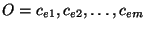
We begin by defining the notation we shall use throughout the
remainder of the paper.
Define an observation as a set of link failures that are
potentially correlated, either temporally or otherwise. In other
words, if a given set of links fail simultaneously
or share a similar pattern or signature of a failure,
these events form an observation.
A hypothesis is a candidate set of circuit failures that could
explain the observation. That is, a hypothesis is a set of risk
groups that contain the set of links seen to fail in a given
observation.
The goal, then, of shared risk group analysis is to obtain a hypothesis that
best explains a given observation. The principle of Occam's razor suggests that
the simplest explanation is the most likely; hence, we consider the best
hypothesis to be the one with the fewest number of risk groups. We note,
however, that there could be other formulations of the problem where a best
hypothesis is optimizing some other metric.
3.1 Problem formulation
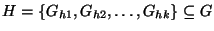
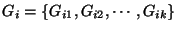
We can define the
problem formally as follows. Given a set of links,
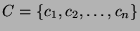 , and risk groups , and risk groups
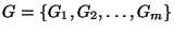 . Each risk group . Each risk group  contains a set of links contains a set of links
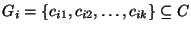 that are likely to fail simultaneously. (We use the terms ``links'' and
``circuits'' here to aid intuition, though it will be apparent that the
formulation and the algorithm to be described simply deals with sets, and can be
applied to arbitrary problem domains). Note that each circuit here can
potentially belong to many different groups. Given an input observation
consisting of events on a subset of circuits, that are likely to fail simultaneously. (We use the terms ``links'' and
``circuits'' here to aid intuition, though it will be apparent that the
formulation and the algorithm to be described simply deals with sets, and can be
applied to arbitrary problem domains). Note that each circuit here can
potentially belong to many different groups. Given an input observation
consisting of events on a subset of circuits,
 , the problem is to identify the most probable hypothesis, , the problem is to identify the most probable hypothesis,
 such that such that  explains explains  , i.e.,
every member of belongs to at least one member of and all the members of
a given group , i.e.,
every member of belongs to at least one member of and all the members of
a given group  belong to . The latter constraint stems from the fact
that if a component fails, all the associated member links fail and hence should
be a part of the observation. is a set cover for ; finding a minimum set
cover is known to be NP complete. belong to . The latter constraint stems from the fact
that if a component fails, all the associated member links fail and hence should
be a part of the observation. is a set cover for ; finding a minimum set
cover is known to be NP complete.
The problem can be modeled visually using a bipartite graph as shown
in Figure 3. Each circuit,  , and group, , and group,  , is
represented by a node in the graph. The bottom partition consists of
nodes corresponding to the risk groups; the top nodes correspond to
circuits. An edge exists between a circuit node and a group node if
that circuit is a member of the risk group. Given this bipartite graph
and a subset of vertices in the top partition (corresponding to an
observation), the problem is to identify the smallest possible set of
group nodes that cover the events. , is
represented by a node in the graph. The bottom partition consists of
nodes corresponding to the risk groups; the top nodes correspond to
circuits. An edge exists between a circuit node and a group node if
that circuit is a member of the risk group. Given this bipartite graph
and a subset of vertices in the top partition (corresponding to an
observation), the problem is to identify the smallest possible set of
group nodes that cover the events.
Before proceeding, we observe that if multiple risk groups have the
same membership--that is, the same set of circuits may fail for two
or more different reasons--it is impossible to distinguish between
the causes. We call any such risk groups aliases, and collapse
all identical groups into one in our set of risk groups. For example,
in Figure 3, group  and and  have the same membership: have the same membership:
 . Hence, and are collapsed into a single group as a
pre-processing step. . Hence, and are collapsed into a single group as a
pre-processing step.
There are potentially many different ways to solve the problem as formulated
above;
we use a greedy approximation to model imperfect fault notifications and
other inconsistencies due to operational realities (as discussed in
). Our greedy approximation also reduces the computation
cost involved in identifying the most likely hypothesis among all hypotheses
(which can potentially be large).
Before presenting the algorithm, however, we must first introduce two metrics we
will use to quantify the utility of a risk group. Let  be the total
number of links that belong to the group be the total
number of links that belong to the group  (known as the cardinality of
). Similarly, (known as the cardinality of
). Similarly,
 is the number of elements of that also
belong to . We define the hit ratio of the group as is the number of elements of that also
belong to . We define the hit ratio of the group as
 . In other words, the hit ratio of a group is the fraction of circuits
in the group that are part of the observation. The coverage ratio of a
group is defined as . In other words, the hit ratio of a group is the fraction of circuits
in the group that are part of the observation. The coverage ratio of a
group is defined as
 . Basically, the coverage ratio is
the portion of the observation explained by a given risk group. . Basically, the coverage ratio is
the portion of the observation explained by a given risk group.
Intuitively, our greedy algorithm attempts to iteratively select the
risk group that explains the greatest number of faults in the
observation with the least error: in other words, the highest coverage
and hit ratios. More concretely, in every iteration, the algorithm
computes the hit ratio and coverage ratio for all the groups that
contain at least one element of the observation (i.e., the
neighborhood of the observation in the bipartite graph). It selects
the risk group with maximum coverage (subject to some restrictions on
the hit ratio which we shall describe later) and prunes both the group
and its member circuits from the graph. In the next iteration, the
algorithm recomputes the hit and coverage ratio for the remaining set
of groups and circuits. This process repeats, adding the group with
the maximum coverage in each iteration to the hypothesis, until
finally terminating when there are no circuits remaining in the
observation.
The pseudocode is presented in Algorithm 1.
![\begin{algorithm}
% latex2html id marker 470
[t]
\caption{greedyHypothesis(input...
...sis, grp);$\ENDWHILE
\STATE $return hypothesis;$\end{algorithmic}\end{algorithm}](img24.png)
![\begin{algorithm}
% latex2html id marker 477
[t]
\caption{findCandidateGroup(gro...
...age(group)$}
\ENDFOR
\STATE {$return maxGroup$}
\end{algorithmic}\end{algorithm}](img25.png)
The algorithm maintains two separate lists: explained and
unexplained. When a risk group is selected for inclusion in the
hypothesis, all circuits in the observation that are explained by this
risk group are removed from the unexplained list and placed in the
explained list. The hit ratio is computed based on the union of the
explained and unexplained list, but coverage ratio is computed based
only on the unexplained list. The reason for this is straightforward:
multiple failures of the same circuit will result in only one failure
observation. Hence, the hit ratio of a risk group should not be
reduced simply because some other risk group also accounts for the
failure observation.
3.3 Modeling imperfections
In our discussion so far, we have skirted the issue of selecting risk
groups with hit ratios less than one. What does it mean to have a
hypothesis that explains more circuit failures than actually occurred?
In a straightforward model, such a result is nonsensical: if the
shared component generating the risk group failed, all constituent
circuits should have been affected. Operational reality, however, is
seemingly contradictory for a number of reasons, including incomplete or erroneous monitoring data, and inaccurate modeling of the shared risk groups.
The failure notices (e.g.,
SNMP traps) are often transmitted using unreliable protocols such as
UDP which can result in partial failure observations. Hence, the
accuracy of the diagnosis can be impacted if the data is erroneous or
incomplete. For example, if due to the failure of a particular optical
component failure, six links went down out of which only five, say,
messages made it to the monitoring system. The hit ratio for the risk
group representing the shared component is then 5/6. Without expressly
allowing for the selection of this risk group, the algorithm would
output a hypothesis, that, while plausible, is likely far from reality.
Furthermore, while theoretically it
should be possible to precisely model all risk groups, it is impossible in
practice to exactly capture all possible failure modes. This difficulty leads to
two interesting cases of inaccurate modeling. One is failure to model high-level
risk groups (e.g., all links terminating in a particular point of presence may
share a power grid) while the other is failure to model low-level risk groups
(for example, some internal risk group within a router). Our algorithm needs to
be robust against imprecise failure groups and, if possible, learn from real
observations. We discuss one real instance of learning of new risk groups from
actual failure observations in Section 6.
We allow for these operational realities by selecting the risk group with
greatest coverage out of those with hit ratios above a certain error threshold.
So, even if a particular circuit is omitted (either due to incorrect modeling or
missing data), the error threshold allows consideration of groups that have most
links but not quite all and cover a large number of failures.
Note that there could be two different cases once we include groups with hit
ratios above a certain error threshold. It is possible that there are genuinely
only few failures but due to information loss the algorithm with no error
threshold outputs a hypothesis with larger number of failures. Relaxing the
error threshold would account for this loss thereby outputting a better (smaller)
hypothesis. On the other hand, there could be genuinely larger number of
failures in which case relaxing the error threshold can output a wrong
hypothesis.
It turns out to be extremely difficult to select a single error threshold for
all observations, as it depends greatly on the size of individual risk groups
involved in the observation. In practice, we run the algorithm multiple times
and generate hypotheses for decreasing error thresholds until a plausible
hypothesis is generated. More generally, we can assign a cost function to
evaluate the confidence of a particular hypothesis based on the number of
component failures in the hypothesis and the threshold used and choose the one
with lowest cost.
Figure 4:
System architecture framework of SCORE.
|
We created SCORE with generality in mind. Accordingly, key systems and
algorithmic components are factored out so that they may be reused in multiple
problem domains or in variations for a single problem domain. A stand-alone
spatial correlation module is driven by an extensible set of problem
domain dependent diagnosis processes. Intelligence from the problem domain is
built into the SRLG database, and is reflected in the SCORE queries.
Figure 4 depicts the SCORE system architecture as it is
implemented today. The following subsections describe the various modules in
more detail.
The SRLG database manages relationships between SRLG
groups and corresponding links. For example, in our application, the database
atoms used to form SRLGs at SONET layer describe SONET level equipment IDs that
particular IP links traverses, extracted from databases populated from
operational optical element management systems. Other risk groups such as area,
router, modules, etc. are similarly formed from the native databases extracted
from the various network elements (e.g. router configurations). We note that
the underlying databases track the network and therefore exhibit churn. The
SCORE software is currently snapshot driven, and copes with churn by reloading
multiple times during the course of the day. As mentioned in
Section 3 on alias aggregation, we collapse risk groups with
identical member links, prior to performing spatial correlation.
4.2 Spatial correlation engine
The Spatial Correlation Engine (SCORE) forms the core of the system. This engine
periodically loads the spatial database hierarchy and responds to queries for
fault localization. SCORE implements the greedy algorithm discussed in
Section 3. That is, SCORE obtains the minimum set hypothesis
using the SRLG database and a given set of inputs. Optionally, an error
threshold can be specified, as described in Section 3.
The set of observations upon which spatial correlation is applied are
obtained from the network fault notifications and performance reports
(including IP performance-related alarms). These in turn come from a wide
range of data sources. We discuss below some of the more popular fault
and performance-related data sources that have been used within the
SCORE architecture to date. Though we describe certain optical layer
event data sources (such as SONET PM data) and have experimented with
such sources with SCORE, only IP event sources were used to obtain the
results described in this paper.
Table 1:
Syslog messages output by Cisco and Avici routers when a link goes down at
different layers of the stack. When the link comes back up, the router writes
similar messages indicating that each of the layer is back up.
pcr
|
Syslog Message on Cisco/Avici Routers |
Layer |
Router |
|
Aug 16 04:01:29.302 EDT: %LINEPROTO-5-UPDOWN: Line protocol on Interface POS0/0,
changed state to down |
SONET layer |
Cisco |
|
Aug 16 04:01:29.305 EDT: %LINK-3-UPDOWN: Interface POS0/0, changed state to down
|
PPP layer |
Cisco |
|
Aug 16 04:01:29.308 EDT: %OSPF-5-ADJCHG: Process 11, Nbr 1.1.1.1 On POS0/0 from FULL to DOWN, Neighbor Down: Interface down or detached
|
OSPF/IP layer |
Cisco |
|
module0036:SUN SEP 12 17:23:29 2004 [030042FF] MINOR:snmp-traps :Sonet link POS 1/0/0 has new adminStatus up and operStatus up. |
Sonet Layer |
Avici |
|
server0001:SUN SEP 12 17:25:01 2004 [030042FF] MINOR:snmp-traps :PPP link POS
1/0/0 has new adminStatus up and operStatus up. |
PPP layer |
Avici |
|
server0002:THU AUG 12 07:21:58 2004 [030042FF] MINOR:snmp-traps:OSPF with
routerId 1.1.1.1 had non-virtual neighbor state change with neighbor
1.1.1.2 (address less 0) (router id 1.1.1.4) to state Down. |
OSPF/IP
layer |
Avici |
|
IP link failures and other faults will be observed by the routers, and reported
to centralized network operations systems via SNMP traps sent from the router.
These SNMP traps provide the key event notifications that allow network
operators to learn of faults as they occur.
Router operating systems, much like Unix operating systems, log important events
as they are observed. These are known as router syslogs and provide a
wealth of useful information regarding network events. These can be used as
additional information to complement the SNMP traps and the alarms that they
generate. Table 1 shows sample Syslog messages for a failure
observed on a Cisco router, and another failure observed on an Avici router. The
failures are reported at different layers--illustrated here for the SONET
layer, PPP layer and IP layer (OSPF). Note that there is no standardized format
for these messages as they are usually output for debugging purposes.
SNMP performance data is generated by
the routers on either a per-interface or per-router basis, as applicable. It
typically contains 5 minute aggregate measurements of statistics such as traffic
volumes, router CPU average utilization, memory utilization of the router,
number of packet errors, packet discards and so on.
Performance metrics are also available on a per circuit
basis from SONET network elements along an optical path (as are alarms, although
these are not discussed here). Numerous parameters will be reported in, for
example, 15 minute aggregates. These include parameters such as coding
violations, errored seconds and severely errored seconds (indicative of bit
error rates and outages), and protection switching counts on SONET rings.
Each of these monitoring data are
usually collected from different network elements (such as routers, SONET DWDM
equipment etc.) and streamed to a centralized database. These different data
are usually stored in different formats with different candidate keys. For
example, the candidate key for SNMP database is an interface number as it
collects interface-level statistics. OSPF messages are based on link IP
addresses. SONET performance monitoring data is based on a circuit identifier.
All these data sources are mapped into link circuit identifiers using a set of
mapping databases.4
4.5 Fault localization policies
Fault localization is performed on various monitoring data sources (such as
those mentioned in the previous section) using flexible data-dependent policies.
In Figure 4, fault isolation policies form the bridge
between the various monitoring data sources (translators) and the main SCORE
engine. These policies dictate how a particular type of fault can be localized.
The main functions include:
-
- Event Clustering. Clustering events that represent either
temporally correlated events or events with similar failure signature (hence
could be spatially correlated)
-
- Localization Heuristics. Heuristics that dictate how to identify the
hypothesis that can best explain these event clusters.
Event Clustering: Data sources that are based on discrete asynchronous
events, (e.g. OSPF messages, Syslog messages) need to be clustered to identify
an observation. This clustering captures all the events that took place in a
fixed time interval as potentially correlated. Note that a failure can have
events that are slightly off in time either due to time synchronization issues
across various elements, or propagation delays in an event to be recorded.
Hence, event clustering has to account for these in recording observations.
There are many different ways to cluster events. A naive approach to clustering
is based on fixed time bins. For example, we can make observations (set of links
potentially correlated) by clustering together all events in a fixed 5 minute
bin. The problem with this approach however is the fact that events related to a
particular failure can potentially straddle the time bin boundary. In this case,
this quantization will create two different observations for correlated events
thus affecting the accuracy of the diagnosis.
In our system, we use a clustering algorithm based on gaps between failure
events. We use the largest chain of events that are spaced apart within a set
threshold (called quiet period) as potentially correlated events. The intuition
here is that two events that occur within a time period less than a given
threshold (say 30 seconds) are potentially correlated and can be attributed to
the same failure. Note however that this particular parameter needs to be tuned
for the particular problem domain. These clustered events are then fed to the
SCORE system to obtain a hypothesis that represents the failed components in the
network.
Although currently we use temporally correlated events as a good indication of
events that potentially can have the same root cause, it is possible to apply
different methods to cluster events. One such alternative method effective for
software bugs where a particular type of router with a particular version of
software might have fault signatures for different links although not
necessarily temporally correlated. An offline analysis tool that can observe
these signatures can then query and find out the risk group associated with
these links.
Localization Heuristics: Fault localization often requires heuristics
that are either derived intuitively or through domain knowledge to make multiple
queries to the system with different parameters in order to obtain higher
confidence hypothesis. SCORE architecture itself allows flexible overlay of
such troubleshooting policies depending on the problem domain. We implemented
one such localization heuristic for handling IP link down events (including
possible database errors).
A simple heuristic we implemented is to query Spatial Correlation engine with
multiple error thresholds (reducing from 1.0 to 0.5) and obtain many different
hypotheses. We compare these hypotheses obtained using different relaxations
(error thresholds) to account for data inconsistencies or database issues. The
most likely hypothesis is based on a cost function that depends on the amount of
error threshold, number of failures in the hypothesis and finally the individual
types of groups in the hypothesis. This policy is more applicable to link
failures identified at the IP layer. Currently we use the ratio between number
of groups and the threshold; we would like to identify cases where a small
relaxation in the threshold (say error threshold of 0.9) can reduce the number
of groups significantly.
Another heuristic is to query the Spatial Correlation engine using clustered
events that have similar signature (e.g. links that had same number of bit
errors in a given time frame). This policy is guided by the intuition that
correlated events in terms of the actual signature potentially have the same
root cause. This heuristic is more suitable to diagnose root-causes of soft
errors in SONET performance monitoring data.
Figure 5:
SCORE screen shot.
|
The main core engine loads (and periodically refreshes) an SRLG database that
has associations from groups to a set of links. It constructs two hashtables,
one for the set of circuits and one for the set of groups. Each group consists
of the circuit identifiers that can be used to query the circuits hashtable.
This particular implementation allows for fast associations and traversals to
implement the spatial correlation algorithm outlined in .
The total implementation of this main SCORE engine is slightly more than 1000
lines of C code. This engine also has a listening server at a particular port on
which various diagnosis agents can connect via popular socket interface and
perform queries on the cluster of link-failures. The SCORE engine then responds
with the hypotheses that can best explain the cluster.
SCORE system is not extremely difficult to implement. Obtaining groups from
different databases that contain fiber level, fiber span level, router level and
other independent databases is one of the functions of the SRLG database module.
This module is implemented in perl and it consists of about 1000 lines of code.
The other function of the SRLG database interface is the group alias resolution.
This group alias resolution algorithm is not a performance bottleneck as it is
refreshed fairly infrequently (usually twice a day) resolution algorithm in
perl. This collapsing of risk groups itself is about 200 lines of perl code.
Clustering events and writing a per-data source event collection module is
written in perl. Finally, the troubleshooting policies themselves need the
flexibility and hence have been implemented in perl too. The total lines of code
for the two policies we implemented is slightly less than a thousand.
The SCORE web interfaces consists of a table consisting of the following
columns. Figure 5 shows a live screenshot of the SCORE web
interface. The interface also allows to view archived logs including raw events
and their associated diagnosis results. The first column outputs the actual
event start time and the end time using one of the clustering algorithms. The
second column represents the set of links that were impacted during the event.
The third and fourth column give descriptions of the groups of components that
form the diagnosis report for that observation. The diagnosis report also
consists of the hit-ratio, coverage ratio and finally error threshold used for
the groups involved in the diagnosis.
Figure 6:
Percentage correct hypotheses as a function of error probability and for various algorithm error
thresholds (three simultaneous failures).
|
We evaluated the performance of the SCORE spatial correlation algorithm using
both artificially generated faults (this section) and real faults (next
section). The main goal of the initial experiments is to evaluate the accuracy
of the greedy approach within a controlled environment by using emulated faults.
We use an SRLG database constructed from the network topology and configuration
data of a tier-1 service provider's backbone. In our simulation, we inject
different number of simultaneous faults into the system and evaluate the
accuracy of the algorithm in obtaining the correct hypothesis. We first study
the efficacy of the greedy algorithm under ideal operating conditions (no losses
in data, no database inconsistencies) followed by the presence of noisy data by
simulating errors in the SRLG database and observations.
5.1 Perfect fault notification
To evaluate the accuracy of the SCORE algorithm, we simulated scenarios
consisting of multiple simultaneous failures and evaluated the accuracy in terms
of the number of correct hypotheses (faults correctly localized by the
algorithm) and the number of incorrect hypotheses (those which we did not
successfully localize to the correct components). We randomly generated a given
number of simultaneous failures selected from the set of all network risk
groups: the set of all SONET components, fiber spans, OSPF areas, routers, and
router ports and modules in our SRLG database. Once the faults were selected
for a given scenario, we identified the union of all the links that belong to
these failures. These link-level failures were then input to the SCORE system
and hypotheses were generated. The resulting hypotheses were then compared with
the actual injected failures to determine those which were correctly identified,
and those which were not.
Figure 6 depicts the fraction of correctly identified hypotheses as a
function of the number of injected faults, where each data point represents an
average across 100 independent simulations. The figure illustrates that the
accuracy of the algorithm on these data sets is greater than 99% for Ports,
Modules and Routers, irrespective of the number of simultaneous failures
generated. In general, the accuracy of the algorithm decreases as the number of
simultaneous failures increases, although the accuracy remains greater than 95%
for less than five simultaneous failures. In reality, it is unlikely that more
than one failure will occur (and be reported) at a single point in time. Thus,
for failures such as fiber cuts, router failures, and module outages
(corresponding to a single simultaneous failure), our results indicate that the
accuracy of the system is near 100%. However, it is entirely possible in a
large network that multiple independent components will simultaneously be
experiencing minor performance degradations, such as error rates, which are
reported and investigated on a longer time scale. Thus, the results
representing higher number of simultaneous failures are likely indicative of
performance troubleshooting. However, we can still conclude that for realistic
network SRLGs, the greedy algorithm presented here is highly accurate when we
have perfect knowledge of our SRLGs and failure observations.
Figure 7:
Percentage correct hypotheses as a function of error probability and for varying number of
simultaneous failures (error threshold = 0.6).
|
Figure 8:
False hypotheses vs error probability (three failures).
|
The SRLG model provides a solid, but not perfect representation of the possible
failure modes within a complex operational network. Thus, we expect to find
scenarios where the set of observations cannot be perfectly described by any
SRLG. Similarly, data loss associated with event notifications and database
errors are inherent operational realities in managing large-scale IP backbones.
In , we discussed how to adapt the basic greedy algorithm to
account for these operational realities. In this section, we evaluate the
accuracy of the SCORE algorithm when we have loss in our observations, which may
result for example from imperfect event notifications (where failures are not
reported for whatever reason). We consider three parameters: the error
threshold used in the SCORE algorithm, the number of simultaneous failures, and
the error probability (which represents the percentage of IP link failure
notifications lost for a given failure scenario).
Figures 7 and 8 demonstrate the
accuracy of the algorithm under a range of error probabilities and algorithm
error thresholds and for different numbers of simultaneous failures.
Specifically, the figures plot the percentage of correct hypotheses as a
function of the error probability. In Figure 7, the
algorithm error threshold is varied from 0.6 to 1.0, whilst the number of
simultaneous failures is set to 3. In Figure 8 the
algorithm error threshold is fixed at 0.6 and the number of simultaneous
failures is varied from 1 to 5. As expected, increasing the error probability
reduces the accuracy of the algorithm. Under three simultaneous failure events
and an error probability of 0.1, we can observe from
Figure 7 that an algorithm error threshold of between 0.7
and 0.8 restores the accuracy of the SCORE algorithm to around 90%. However, if
we mandate perfect matching of failure observations to SRLGs (i.e., error
threshold = 1.0), then our accuracy in isolating our fault drops to around 78%.
This shows the necessity and effectiveness of the of the error thresholds
introduced into the algorithm for fault localization in the face of noisy event
observation data.
The algorithm's execution time was also evaluated under a range of
conditions. In general, the execution time recorded increased as the
number of IP links (observations) impacted by the failures increased.
This is because all of the SRLGs associated with each of the failed
links must be included as part of the candidate set of SRLGs for
localization, and thus must be evaluated. Thus, the execution time
increased within increasing numbers of failures, but on average was
below 150 ms for up to ten failures. Similarly, the execution time
for scenarios involving router failures was typically higher than for
other failure scenarios, as the routers typically involved larger
numbers of links. Execution times of up to 400 ms were recorded for
events involving large routers. However, even in these worst case
scenarios, the algorithm is more than fast enough for real-time
operational environments.
6 Experience in a tier-1 backbone
Table 2:
Summary of real, tier-1 backbone failures successfully diagnosed by SCORE.
|
Type of |
Component |
#SRLGS |
Final Thld |
#SRLGS |
#Correctly |
#Incorrectly |
Comment |
|
problem |
Name |
(Thld.=0.6) |
|
(Thld.=Final) |
localized |
localized |
|
| Router |
Router A |
27 |
0.8 |
1 |
1 |
0 |
No event reported by some
links |
|
Router |
Router B |
20 |
0.9 |
3 |
3 |
0 |
No event reported by some
links |
|
Router |
Router C |
12 |
0.7 |
1 |
1 |
0 |
No event reported by some
links |
|
Router |
Router D |
1 |
1 |
1 |
1 |
0 |
- |
|
Router |
Router E |
18 |
0.8 |
1 |
1 |
0 |
No event reported by some
links |
|
Router |
Router F |
1 |
1 |
1 |
1 |
0 |
- |
|
Router |
Router G |
4 |
1 |
4 |
4 |
0 |
- |
| Module |
Module A |
1 |
1 |
1 |
1 |
0 |
- |
|
Module |
Module B |
1 |
1 |
1 |
1 |
0 |
- |
|
Module |
Module C |
1 |
1 |
1 |
1 |
0 |
- |
| Optical |
Sonet A |
8 |
0.9 |
2 |
1 |
1 |
No observation reported
by one link and database problem |
|
Failed Transceiver |
Sonet B |
1 |
1 |
1 |
1 |
0 |
- |
|
Short term Flap |
Sonet C |
2 |
0.7 |
1 |
1 |
0 |
No observation reported
by one link |
|
Optical Amplifier |
Sonet D |
2 |
0.6 |
1 |
1 |
0 |
No observation reported
by one link |
| Fiber Cut |
Fiber A |
3 |
0.5 |
1 |
1 |
2 |
Database problem |
|
Fiber Span |
Fiber Span A |
1 |
1 |
1 |
1 |
0 |
- |
| Protocol Bug |
OSPF Area A |
20 |
0.7 |
4 |
4 |
0 |
Incorrect SRLG modeling |
|
Protocol Bug |
OSPF Area A |
4 |
1 |
4 |
4 |
0 |
OSPF Area A MPLS enabled interfaces |
|
|
|
|
|
|
|
|
|
The SCORE prototype implementation was recently deployed in a tier-1
backbone network, and used in an offline fashion to isolate IP link
failures reported in the network. The implemented system operated on a
range of fault and performance data, including IP fault notifications
and optical layer performance measures. However, we limit our
discussion here to our experience with link failure events reported in
router syslogs.
Determining whether or not the SCORE prototype correctly localized a
given fault requires identification of the root cause of the fault via
other means. In many cases, identifying this root cause involved
sifting through large amounts of data and reports--a tedious process
at best. We were able to manually confirm the root cause of 18 faults;
we present a comparison with the output reported by the SCORE
prototype. We note, however, that our methodology has an inherent
bias: we cannot exclude the possibility that there may be a
correlation (not necessarily positive) between our ability to diagnose
the fault and SCORE's performance. While it would have been
preferable to select a subset of the faults at random, we were not
able to manually diagnose every fault, nor did we have the resources
to consider all faults experienced during SCORE's deployment.
Table 2 denotes the results of our analysis of each of our
18 faults.
For each failure scenario, we report:
-
- the type of failure that occurred
-
- a name uniquely identifying the failed component
-
- the number of SRLG groups localized when the algorithm was run with a threshold of 1.0
-
- the threshold used to generate a final conclusion
-
- the number of SRLGs localized when the algorithm was run with the final threshold
-
- the number of SRLGs correctly localized
-
- the number of SRLGs incorrectly localized
-
- description of the reason why we had to reduce the threshold, or why we were unable to identify a single
SRLG as the root cause in certain situations
Overall, we were able to successfully localize all of the faults studied to the
SRLGs in which the failed network elements were classified--except where we
encountered errors in our SRLG database. However, when we used a threshold of
1.0 (i.e., mandated that an SRLG can be identified if and only if faults were
observed on all IP links), then we were typically unsuccessful--particularly
for router failures, and for the protocol bug reported. In the majority of the
router failures, even though these events corresponded to routers being
rebooted, the remote ends of the links terminating on these routers did not
always report associated link-level events. This may be due to a number of
possible scenarios: the events may never have been logged in the syslogs, data
may have been lost from the syslogs, the links may have been operationally shut
down and hence did not fail at this point in time, or the links were
not impacted by the reboot. Independent of why the link notifications were not
always observed, the router failures were all successfully localized when the
threshold was marginally reduced. This highlights the importance of the
threshold concept in the SCORE algorithm to localize faults in operational
networks.
Of course, router failures are typically easy to identify through spatial
correlation, as all of the links impacted have a common end point (the failed
router). However, optical layer impairments can impact seemingly logically
independent links at the IP layer if these links are all routed through a common
optical component, making them much more difficult to identify.
We study four different SONET network element failures. The first--an optical
amplifier failure--induced faults reported on 13 IP links. Thus, with a
threshold of 1.0 our algorithm identified 8 different SRLGs as being involved.
However, as the threshold was reduced to 0.9, we were able to isolate the fault
to only 2 different SRLGs. Further reductions in this threshold did not,
however, further reduce the number of SRLGs to which the fault was localized.
Further investigation uncovered an SRLG database problem--where our SONET
network element database did not contain any information regarding one of the
circuits reporting the fault. Thus, the SCORE algorithm was unable to localize
the fault for this particular IP link to the SRLG containing the failed optical
amplifier, and instead incorrectly concluded that a router port was also
involved (the second SRLG). However, the SRLG containing the failed amplifier
was also correctly identified for the other 12 IP links--the lower threshold
was required because no fault notification was observed for one of the IP links
routed through the optical amplifier.
This optical amplifier example highlights a particularly important capability of
the SCORE system--the ability to highlight potential SRLG database errors.
Links missing from databases, incorrect optical layer routing information
regarding circuits and other potential errors in databases play havoc with
capacity planning and network operations and so must be identified. In this
scenario, the database error was highlighted by the fact that we were unable to
identify a single SRLG for a single network failure, even after lowering
threshold using in the SCORE algorithm.
The other three SONET failures were all correctly isolated to the SRLG
containing the failed network element, in two cases we again had to lower the
threshold used within the algorithm to account for links for which we had no
failure notification (in one of these cases, the missing link was indeed a
result of the interface having been operationally shut down before the failure).
We tested our SCORE prototype on a second, previously identified failure
scenario impacted by a SRLG database error (fiber A in
table 2). Again, the SCORE system was unable to identify a
single SRLG as being the culprit even as the threshold was lowered--as no SRLG
in the database contained all of the circuits reporting the fault. So again, a
database error was highlighted by the inability of the system to correlate the
failure to a single SRLG.
The final case that we evaluated was one in which a low level protocol
implementation problem (commonly known as a software bug!) impacted a number of
links within a common OSPF area. This scenario occurred over an extended period
of time, during which three other independent failures were simultaneously
observed in other areas.
When a threshold of 1.0 was used in the SCORE algorithm, the event in question
was identified as being the result of 20 independent SRLG failures--a large
number even for the extended period of time! As the threshold was reduced to a
final value of 0.7, the event was isolated to four individual SRLGs--three
SRLGs in other OSPF areas (corresponding to the independent failures) and the
OSPF area in question. Thus, the SCORE algorithm was correctly able to identify
that the event corresponded to a common OSPF area. However, further
investigation uncovered that the reason why not all links in the OSPF area were
impacted was that only those interfaces that were currently MPLS-enabled were
affected. Thus, an additional SRLG was added to our SRLG database that
incorporated the links in a given area that were MPLS enabled--application of
this enhanced SRLG database successfully localized all of the SRLGs impacted by
the four simultaneous failures with a threshold of 1.0. Thus, this illustrates
how the threshold used in the SCORE algorithm can allow our results to be robust
to incomplete modeling of all of the possible SRLGs--any level of modeling of
risk groups can be inadequate as there could be more complicated failure
scenarios that cannot be modeled by humans perfectly a priori. However, we also
illustrated how we can continually learn new SRLGs through further analysis of
new failure scenarios, thereby enhancing our SRLG modeling.
While the 18 faults we have studied
demonstrate the ability of SCORE to correctly localize faults, it does not give
an indication about how much we could localize. In this section, we evaluate the
efficiency of SCORE using a metric we call localization efficiency. The
localization efficiency of a given observation is defined as the ratio of the
number of components after localization to that before localization. In other
words, it is the fraction of components that are likely to explain a particular
fault (or observation) using our localization algorithm out of all the
components that can cause a given fault.
Define
 as the set of groups that a circuit
belongs to. is an observation consisting of circuits as the set of groups that a circuit
belongs to. is an observation consisting of circuits
 . The most probable hypothesis . The most probable hypothesis
 is
the hypothesis output by the algorithm. Then, localization efficiency is given by is
the hypothesis output by the algorithm. Then, localization efficiency is given by
 . .
Figure 9:
CDF of localization efficiency out of about 3000 real faults we have
been able to localize.
|
In Figure 9, the cumulative distribution function of the
localization efficiency is shown. From the Figure 9, we can
clearly observe that SCORE could localize faults to less than 5% for more than
40% of the failures and to less than 10% for more than 80% of the failures.
This clearly demonstrates that SCORE can identify likely root causes very
efficiently out of a large set of possible causes for a given failure.
Network engineers commonly employ the concept of Shared Risk Link
Groups (SRLGs) to disjoint paths in optical networks, and serve as a
key input into many traffic engineering mechanisms and protocols such
as Generalized Multi-Protocol Label Switching (GMPLS). Due to their
importance, there has been a great deal of recent work on
automatically inferring SRLGs [20]. To the best of our
knowledge, however, we are the first to use SRLGs in combination with
IP-layer fault notifications to isolate failures in the optical
hardware of a deployed network backbone without the need for
monitoring at the physical layer.
Monitoring and management is a challenging problem for any large
network. It is not surprising, then, that a number of research
prototypes [17,3,15,16,6,10]
and commercial products have been developed to diagnose problems in IP
and telephone networks. Commercial network fault management systems
such as SMARTS [21], OpenView [12],
IMPACT [13], EXCpert [16],
and NetFACT [11] provide powerful, generic frameworks for
handling fault indicators, particularly diverse
SNMP-based [2] measurements, and rule-based correlation
capabilities. These systems present a unified reporting interfaces to
operators and other production network management systems. In
general, however, they correlate alarms from a particular layer in
order to isolate problems at that same layer (e.g., route flapping,
circuit failure, etc.).
Roughan et. al. propose a correlation-based approach to detect
forwarding anomalies including BGP-related
anomalies [19]. Their approach was to detect events
of potential interest by correlating multiple data sources while our
approach was to diagnose these events to identify root causes.
The problem of fault isolation is obviously not limited to networking;
similar problems exist in any complex system. Regardless of domain,
fault detection systems have taken three basic approaches: rule or
model-based reasoning [12,1,7], codebook
approaches [21,25], or machine learning (such as Bayesian
or Belief Networks [24,22,5]).
The difficulty with probabilistic or machine learning approaches is
that they are not prescriptive: it's not clear what sets of scenarios
they can handle besides the specific training data. Rule-based and
codebook systems (otherwise known as ``expert systems'') are often
even more specific, only being able to diagnose events that are
explicitly programmed. Model-based approaches are more general, but
require detailed information about the system under test.
Dependency-based systems like ours, on the other hand, allow general
inference without requiring undue specificity. Indeed, the specific
use of dependency graphs for problem diagnosis has been explored
before [9], but not in this particular domain.
Our problem as defined in falls into the more
general class of inference problems which include problems in other domains such
as traffic matrix estimation, tomography, etc. Hence, techniques applied in
these domains can be potentially used to solve this problem. For example, in
[26], the authors reduce the problem of traffic matrix
estimation to an ill-posed linear inverse problem and apply a regularization
technique to estimate the traffic matrix. Similarly, our problem also can be
solved using matrix inversion methods, using an incidence matrix to model the
risks. While these methods can work well with perfect data, it is unclear how to
adapt these techniques to deal with imperfect loss notifications and SRLG
database errors. Besides, our greedy approximation works with an accuracy of
over 95% for a large class of failures as shown in our evaluation
().
Hence, the additional benefit in applying any other technique to solve the
problem is only marginal.
Using our risk modeling methodology, we have developed a system that
accurately localizes failures in an IP-over-optical tier-1 backbone.
Given a set of IP-layer events occurring within a small time window,
our heuristics pinpoint the shared risk (optical device) that best
explains these events. Given the harsh operational reality of
maintaining complex associations between objects in the two networking
layers in separate databases, we find that it is necessary to go
beyond identifying the single best explanation, and, instead, to
generate a set of likely explanations in order to be robust to
transient database glitches.
We put forward a simple, threshold-based scheme that looks for best
explanations admitting inconsistencies in the data underlying the
explanations up to a given threshold. We find that not only does this
increase the accuracy and robustness of fault localization, it also
provided a new capability for identifying topology database problems,
for which we had no alternative automated means of detecting. Getting
shared risk information right is critical to IP network design. For example, a
misidentification of a shared risk might produce a design believed to
be resilient to single SRLG failure which in fact is not.
This paper benefitted greatly from discussions with Jennifer Rexford, Aman
Shaikh, Sriram Ramabhadran, Laurie Knox, Keith Marzullo, Stefan Savage, comments
from the anonymous reviewers and our shepherd, Vern Paxson.
- 1
-
S. Brugbosi, G. Bruno, et al.
An Expert System for Real-Time Fault Diagnosis of the Italian
Telecommunications Network.
In Proc. 3rd International Symposium on Integrated Network
Management, pages 617-628, 1993.
- 2
-
J. Case, M. Fedor, M. Schoffstall, and J. Davin.
A Simple Network Management Protocol (SNMP).
In RFC 1157, May 1990.
- 3
-
C. S. Chao, D. L. Yang, and A. C. Liu.
An automated fault diagnosis system using hierarchical reasoning and
alarm correlation.
Journal of Network and Systems Management, 9(2):183-202, 2001.
- 4
-
S. Chaudhuri, G. Hjalmtysson, and J. Yates.
Control of lightpaths in an optical network, Jan. 2000.
IETF draft-chaudhuri-ip-olxc-control-00.txt.
- 5
-
M. Chen, A. Zheng, J. Lloyd, M. I. Jordan, and E. Brewer.
A statistical learning approach to failure diagnosis.
In Proc. International Conference on Autonomic Computing
(ICAC-04), May 2004.
- 6
-
R. H. Deng, A. A. Lazar, and W.Wang.
A probabilistic approach to fault diagnosis in linear lightwave
networks.
In Integrated Network Management III, pages 697-708, Apr.
1993.
- 7
-
G. Forman, M. Jain, M. Mansouri-Samani, J. Martinka, and A. C. Snoeren.
Automated whole-system diagnosis of distributed services using
model-based reasoning.
In Proc. 9th IFIP/IEEE Workshop on Distributed Systems:
Operations and Management, Oct. 1998.
- 8
-
GenSym.
Integrity.
https://www.gensym.com.
- 9
-
B. Gruschke.
Integrated event management: Event correlation using dependency
graphs.
In Proc. 9th IFIP/IEEE Workshop on Distributed Systems:
Operations and Management, Oct. 1998.
- 10
-
P. Hong and P. Sen.
Incorporating non-deterministic reasoning in managing heterogeneous
network.
In Integrated Network Management II, pages 481-492, Apr.
1991.
- 11
-
K. Houck, S. Calo, and A. Finkel.
Towards a Practical Alarm Correlation System.
In Proc. 4th IEEE/IFIP Symposium on Integrated Network
Management, 1995.
- 12
-
HP Technologies Inc.
Open View.
https://www.openview.hp.com.
- 13
-
G. Jakobson and M. D. Weissman.
Alarm correlation.
IEEE Network, 7(6):52-59, Nov. 1993.
- 14
-
I. P. Kaminow and T. L. Koch.
Optical Fiber Telecommunications IIIA.
Academic Press, 1997.
- 15
-
G. Liu, A. K. Mok, and E. J. Yang.
Composite events for network event correlation.
In Integrated Network Management VI, pages 247-260, 1999.
- 16
-
Y. A. Nygate.
Event correlation using rule and object based techniques.
In Integrated Network Management, IV, pages 278-289.
- 17
-
P.Wu, R. Bhatnagar, L. Epshtein, M. Bhandaru, and Z. Shi.
Alarm correlation engine (ACE).
In Proc. Network Operation and Management Symposium, pages
733-742, 1998.
- 18
-
R. Ramaswami and K. Sivarajan.
Optical Networks: A Practical Perspective.
Academic Press/Morgan Kaufmann, Feb. 1998.
- 19
-
M. Roughan, T. Griffin, Z. M. Mao, A. Greenberg, and B. Freeman.
Combining routing and traffic data for detection of ip forwarding
anomalies.
In Proc. ACM SIGCOMM NeTs Workshop, Aug. 2004.
- 20
-
P. Sebos, J. Yates, D. Rubenstein, and A. Greenberg.
Effectiveness of shared risk link group auto-discovery in optical
networks.
In Proc. Optical Fiber Communications Conference., Mar. 2002.
- 21
-
SMARTS.
InCharge.
https://www.smarts.com.
- 22
-
M. Steinder and A. Sethi.
End-to-end Service Failure Diagnosis Using Belief Networks.
In Proc. Network Operation and Management Symposium, Florence,
Italy, Apr. 2002.
- 23
-
J. Strand, A. Chiu, and R. Tkach.
Issues for routing in the optical layer.
In IEEE Communications, Feb. 2001.
- 24
-
H. Wietgrefe, K. Tochs, et al.
Using Neural Networks for Alarm Correlation in Cellular Phone
Networks.
In Proc. International Workshop on Applications of Neural
Networks in Telecommunications, 1997.
- 25
-
S. A. Yemini, S. Kliger, E. Mozes, Y. Yemini, and D. Ohsie.
High speed and robust event correlation.
IEEE Communications, 34(5):82-90, 1996.
- 26
-
Y. Zhang, M. Roughan, C. Lund, and D. Donoho.
An Information-Theoretic Approach to Traffic Matrix Estimation.
In Proc. ACM SIGCOMM, 2003.
IP Fault Localization Via Risk Modeling
This document was generated using the
LaTeX2HTML translator Version 2002 (1.62)
Copyright © 1993, 1994, 1995, 1996,
Nikos Drakos,
Computer Based Learning Unit, University of Leeds.
Copyright © 1997, 1998, 1999,
Ross Moore,
Mathematics Department, Macquarie University, Sydney.
The command line arguments were:
latex2html -split 0 -show_section_numbers -local_icons paper.tex
The translation was initiated by Ramana Rao Kompella on 2005-04-01
Footnotes
... databases.4
We map all the databases into link circuit
identifiers since the network database itself is organized based on link circuit
identifiers. However, any unified format would work equally well.
Ramana Rao Kompella
2005-04-01
|

![\includegraphics[width=0.6\textwidth]{fp_correct.eps}](img28.png)
![\includegraphics[width=0.6\textwidth]{fail_errorp.eps}](img29.png)
![\includegraphics[width=0.6\textwidth]{localization.eps}](img35.png)
![\includegraphics[width=0.6\textwidth]{srlg.eps}](img2.png)
![\includegraphics[width=0.6\textwidth]{stats.eps}](img3.png)
![\includegraphics[width=0.6\textwidth]{theory.eps}](img4.png)
![\includegraphics[width=0.6\textwidth]{score.eps}](img26.png)
![\includegraphics[width=0.6\textwidth]{screenshot.eps}](img27.png)
![\includegraphics[width=0.6\textwidth]{hypo_errorp.eps}](img30.png)