Adaptive nature of SARC

Figure 7: A comparison of cache space allocated to SEQ list by LRU Top, LRU Bottom, and SARC for the SPC-1 Like workload in cache-sensitive configuration. The vertical lines demarcate the high load schedule in Table I.

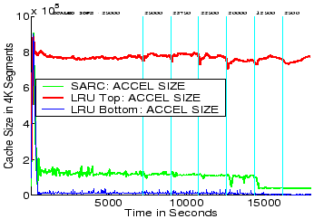
The Figure 7 plots the sizes of the SEQ list versus the time (in seconds) for all the three algorithms. It can be seen that LRU Top allocates too much cache space to SEQ list, LRU Bottom allocates too little cache space to SEQ list, while SARC adaptively allocates just the right amount of cache space to SEQ so as improve the overall performance. It can also be seen that SARC adapts to the evolving workload and selects a different size for the SEQ list at different loads.

Figure 8: A comparison of the quantity $(2 \cdot s \cdot \Delta L)/L$ for LRU Top, LRU Bottom, and SARC for the SPC-1 Like workload in cache-sensitive configuration. The vertical lines demarcate the high load schedule in Table I.

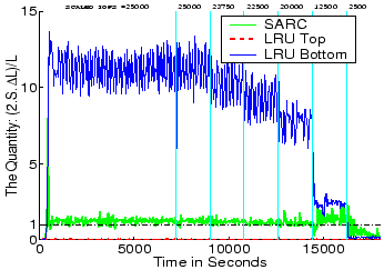The Figure 8 plots the quantity $(2 \cdot s \cdot \Delta L)/L$ for the three algorithms. This quantity is denoted by variable ${\sf ratio}$ in line 4 of the algorithm in Figure 4. It can be seen that for LRU Bottom keeps ${\sf ratio}$ too large meaning that it would benefit by further increase in cache space devoted to sequential data. Similarly, LRU Top keeps ${\sf ratio}$ too small meaning that it would benefit by a decrease in cache space devoted to sequential data. Whereas SARC keeps ${\sf ratio}$ to roughly the idealized value of $1$ meaning that it essentially gets very close to the optimum. In other words, SARC will not benefit by further trading of cache space between SEQ and RANDOM, whereas the other two algorithms would. This plot clearly explains why SARC outperforms the LRU variants in the top three panels of Figure 7. Furthermore, quite importantly, this plot also indicates that any other algorithm that does not directly attempt to drive ${\sf ratio}$ to $1$ as SARC does will not be competitive with SARC. For example, any algorithm that keeps sequential data in the cache for a fixed time [1] or allocates a fixed, constant amount of space to sequential data [29], cannot in general outperform SARC.

Remark 4.1   For heavy sequential workloads, SARC keeps SEQ list just as large enough as useful and does not starve the random workload if present. If there is no random workload then the entire cache will be devoted to the sequential workload and vice versa. When both heavy sequential and heavy random workloads are present, SARC computes the marginal utility to dynamically divide the cache between the two workloads.