Improving Sketch Reconstruction Accuracy
Using Linear Least Squares Method

Gene Moo Lee, Huiya Liu, Young Yoon and Yin Zhang
Department of Computer Sciences
University of Texas at Austin
Austin, TX 78712, USA
{gene,huiyaliu,agitato7,yzhang}@cs.utexas.edu

Abstract:

Sketch is a sublinear space data structure that allows one to approximately reconstruct the value associated with any given key in an input data stream. It is the basis for answering a number of fundamental queries on data streams, such as range queries, finding quantiles, frequent items, etc. In the networking context, sketch has been applied to identifying heavy hitters and changes, which is critical for traffic monitoring, accounting, and network anomaly detection.

In this paper, we propose a novel approach called lsquare to significantly improve the reconstruction accuracy of the sketch data structure. Given a sketch and a set of keys, we estimate the values associated with these keys by constructing a linear system and finding the optimal solution for the system using linear least squares method. We use a large amount of real Internet traffic data to evaluate lsquare against countmin, the state-of-the-art sketch scheme. Our results suggest that given the same memory requirement, lsquare achieves much better reconstruction accuracy than countmin. Alternatively, given the same reconstruction accuracy, lsquare requires significantly less memory. This clearly demonstrates the effectiveness of our approach.

1 Introduction

For many network management applications, it is essential to accurately monitor and analyze network traffic. For example, Internet service providers need to monitor the usage information in order to support usage-based pricing. Network operators need to observe the traffic pattern to perform traffic engineering. Network anomaly detection systems need to continuously monitor the traffic in order to uncover anomalous traffic patterns in near real-time, especially those caused by flash crowds, denial-of-service attacks (DoS), worms, and network element failures. These applications typically treat the traffic as a collection of flows with some properties to keep track of (e.g., volume, number of packets). The flows are typically identified by certain combination of packet header fields (e.g., IP addresses, port numbers, and protocol).

A naïve approach for network traffic measurement is to maintain state and perform analysis on a per-flow basis. However, as link speeds and the number of flows increase, keeping per-flow state can quickly become either too expensive or too slow. As a result, a lot of recent networking research efforts have been directed towards developing scalable and accurate techniques for performing traffic monitoring and analysis without keeping per-flow state (e.g., [6]). Meanwhile, computation over massive data streams has been an active research area in the database research community over the past several years. The emerging field of data stream computation deals with various aspects of computation that can be performed in a space- and time-efficient manner when each item in a data stream can be accessed only once (or a small number of times). A rich body of algorithms and techniques have been developed. A good survey of the algorithms and applications in data stream computation can be found in [11].

A particularly powerful technique is sketch [1,7,3,5], a probabilistic summary data structure proposed for analyzing massive data streams. Sketches avoid keeping per-flow state by dimensionality reduction techniques, using projections along random vectors. Sketches have some interesting properties that have proven to be very useful in analyzing data streams: they are space efficient, provide provable probabilistic reconstruction accuracy guarantees, and are linear (i.e., sketches can be combined in an arithmetical sense). These properties have made sketch the basis for answering a number of fundamental queries on data streams, such as range queries, finding quantiles and frequent items [11]. In the networking context, sketch has been successfully applied to detecting heavy hitters and changes [8,4].

A key operation on the sketch data structure is so called point estimation, i.e., to estimate the accumulated value associated with a given key. All existing methods perform point estimation for different keys separately and only have limited accuracy. In this paper, we propose a novel method called lsquare to significantly improve the accuracy of point estimation on the sketch data structure. Instead of estimating values for individual keys separately, lsquare first extracts a set of keys that is a superset of all the heavy hitter flows and then simultaneously estimates the accumulated values for this set of keys - it does so by first constructing a linear system and then finding the optimal solution to the system through linear least squares method.

We use a large amount of real Internet traffic data to evaluate our method against countmin [5], the best existing sketch scheme. Our results are encouraging: Given the same memory requirement, lsquare yields much more accurate estimates than countmin; and given the same reconstruction accuracy, lsquare uses significantly less memory.

The remainder of the paper is organized as follows. In Section 2, we give an overview of sketch data structure, define the problem, and survey the related work. In Section 3, we describe our lsquare method for point estimation on the sketch data structure. In Section 4, we evaluate the proposed method using real Internet traffic data. We conclude in Section 5.

2 Background

This section provides some background on the problem we want to solve. First, we briefly describe the underlying data stream model and the sketch data structure. Then we define the problem of point estimation on sketch and explain the existing methods to solve the problem. We will also briefly survey the related work.

2.1 Data Stream Model

Let $\mathcal{I} = (k_1,u_1), (k_2, u_2), \ldots$ be an input stream that arrives sequentially, item by item. Here $k_t \in \{0, \ldots, {n-1}\}$ is a key and $u_t \ge 0$ is the update value associated with the key. Let $U_{k}$ be the sum of update values for a key $k$. Here, the update values are non-negative, meaning that $U_k$ always increase. This model is called the cash register model [11]. Many applications of sketches guarantee that counts are non-negative. However, we note that our proposed method is also applicable to the more general Turnstile model [11], in which update values may be negative.

2.2 Count-Min Sketch

Sketch [5,8,14] is a sublinear space data structure for summarizing massive data streams. We use the notations in Table 1 to specify the sketch data structure.

Data structure: A sketch is a two-dimensional count array $T[i][j]$ ( $0 \leq i < H, 0 \leq j < K$), where $H$ is the number of one-dimensional arrays and $K$ is the number of counts in each array. Each count of sketch is initially set to zero. For each one-dimensional array $T[i][\cdot]$, there is a hash function $h_i : \{0, \ldots,{n-1}\} \to \{0, \ldots,{K-1}\}$, where $n$ is the size of the key space. The hash functions are chosen uniformly at random to be pair-wise independent. We can view the data structure as an array of hash tables.

Update procedure: When an update $(k_t, u_t)$ arrives, the update value $u_t$ is added to the corresponding count $T[i][h_i(k_t)]$ in each hash table $i$.

Heavy hitter identification: Since the sketch data structure only records the values, not the keys, it is a challenge to identify the heavy-valued keys among all the keys hashed into the heavy buckets. In order to identify heavy hitters, we can keep a priority queue to record the top hitters with values above $\theta$ (as shown in [5]). An alternative is to perform intersections among buckets with heavy counts, which is proposed by Schweller et al. [14].

Point estimation: Let $S$ be a sketch and $X$ be a set of keys, which are known to be heavy hitters. The problem of point estimation is to estimate the total update value $U_{k}$ for any key $k \in X$. This problem is the focus of our paper.

Count-Min: As proposed in [5], countmin is an existing method to reconstruct the value for any given key. The minimum value among all counts corresponding to the key is taken as an estimate of the value. Formally,

$$U_{k}^{\mathrm{countmin}} = \min_{0 \leq i < H} T[i][h_i(k)]$$

is an estimate for the value $U_k$. Cormode and Muthukrishnan [5] proved that $U_{k} \leq U_{k}^{\mathrm{countmin}}$ and that $U_{k}^{\mathrm{countmin}} \leq U_{k} + \epsilon \Vert \mathbf{U} \Vert _1$ with probability $\delta$, where $H = \lceil \frac{\mathbf{e}}{\epsilon} \rceil$, $K = \lceil \ln \frac{1}{\delta} \rceil$, and $\Vert \mathbf{U} \Vert _1 = \sum_{k=0}^{n-1} \vert U_{k} \vert$. In other words, countmin always overestimates with a certain error bound.

Table 1: Sketch Notations

$H$	number of hash tables
$K$	number of counts per hash table
$n$	size of the key space
$h_i$	$i^{\mathrm{th}}$ hash function
$T[i][j]$	bucket $j$ in hash table $i$
$\theta$	threshold of heavy hitters
$m$	number of top hitters

2.3 Related Work

Common applications of sketches include detecting heavy-hitters, finding quantiles, answering range/point queries and estimating flow size distribution [11].

Kumar et al. [9] used Expectation Maximization method to infer the flow size distribution from an array of counters, which can be viewed as a special case of sketch ($H=1$).

Estan and Varghese [6] suggested an improved sampling method called sample-and-hold, with which flow amount is recorded only after individual entry for the flow is made. They also proposed multi-stage filters for data summary, which has the same data structure as sketch but uses a different update method called conservative update. When an update arrives, only the minimum valued bucket is incremented, whereas sketch increments counters of $all$ corresponding buckets. The minimum counter of multi-stage filter can be used for point estimation, which is similar to the countmin approach.

Krishnamurthy et al. [8] proposed another point estimation method for sketch, which can be used in the Turnstile data stream model. The estimation $U_k^{\mathrm{est}}$ for a key $k$ is given as $U_k^{\mathrm{est}} = \textrm{median} \{ U_k^{i} \vert  0 \leq i < H \}$, where $U_k^{i} = \frac{T[i][h_i(k)] - SUM/K}{1 - 1/K}$ and $SUM = \sum_{j=0}^{K-1} T[0][j]$.

3 Our Approach

In this section, we explain the proposed lsquare method for point estimation. First, lsquare records the data flow information in a sketch. Then it constructs a linear system based on the sketch, and solves the system using linear least squares method. Below we first give a simple example and then formally describe the method.

3.1 A Simple Example

Suppose we have a data stream from $5$ IP addresses. Let $U_{0}=5, U_{1}=4, U_{2}=3, U_{3}=9, U_{4}=16$ be the total amount of traffic for each IP. We record the flows into a sketch with $H=2$ and $K=3$, which has two hash functions $h_1(k) = k \bmod 3$ and $h_2(k) = (k \oplus 3) \bmod 3$, where $\oplus$ denotes bitwise-XOR. The sketch is given as:

$$\begin{tabular}{\vert c\vert c\vert c\vert c\vert} \cline{2-4} \m... ...line $T[1][j]$ & $14^{0,3}$ & $19^{2,4}$ & $4^{1}$ \\ \hline \end{tabular}$$

Here, $14^{0,3}$ means that $U_0$ and $U_3$ are hashed into the bucket, resulting in a count of $14$. The goal is to reconstruct $U_{3}$ and $U_{4}$ from the sketch.

Solution using countmin: $U_{3}^{\mathrm{countmin}}$ = min{$T[0][0]$, $T[1][0]$} = 14 and $U_{4}^{\mathrm{countmin}}$ = min{$T[0][1]$, $T[1][1]$} = 19.

Solution using lsquare: First, we construct a linear system $A \mathbf{x}= \mathbf{b}$ with the constructed sketch. Vectors $\mathbf{x}$, $\mathbf{b}$ and matrix $A$ are specified as follows.

$${%\scriptsize \mathbf{x} = \left[ \begin{array}{c} x_{3} \ x_{4}... ...\ 0 & 0 & 1 \ 1 & 0 & 1 \ 0 & 1 & 1 \ 0 & 0 & 1 \\ \end{array} \right]. }$$

Here, $x_3$ and $x_4$ are variables for keys $3$ and $4$, and $y$ is used to capture noise caused by keys that are not of our interest. Matrix $A$ indicates which keys are hashed to which buckets, and vector $\mathbf{b}$ consists of values of all buckets. For example, we have the equation $x_3 + y = 14$ with bucket $T[0][0]$, which corresponds to the first rows of $A$ and $\mathbf{b}$.

With the constructed linear system, we find the optimal solution of the linear system using linear least squares method: $\mathbf{x} = [10.5, 16.0, 3.5]^T$ (i.e., $x_3 = 10.5$, $x_4 = 16.0$, $y = 3.5$). In this simple example, our method clearly produces much more accurate estimates than countmin.

3.2 Formal Description of lsquare

Let $S$ be a sketch and $k_1, \ldots , k_m$ be the set of keys of our interest. Then we have an unknown variables vector $\mathbf{x} \in \mathbb{R}^{(m+1) \times 1} = [x_{1}, \ldots, x_{m}, y]^T$, where $x_i$ is for the value of key $k_i$ and $y$ is an additional variable for noise caused by keys not in $\{ k_i \}$, which is uniformly distributed over all buckets. We construct a matrix $A \in \{0, 1\}^{{HK} \times (m+1)}$, showing which keys are hashed into which buckets, and a vector $\mathbf{b} \in \mathbb{R}^{{HK} \times 1}$, containing values of every buckets. The elements of $A$ and $\mathbf{b}$ are specified as follows. For $i \in \{0, \ldots {H-1}\}$ and $j \in \{0, \ldots {K-1}\}$,

$$A_{Ki+j+1,\ell} = \left\{ \begin{array}{ll} 1 & \textrm{if key $k_\ell$ is hashed ... ... 1 & \textrm{if $\ell = m+1$,} \\ 0 & \textrm{otherwise,} \end{array} \right.$$

$$b_{Ki+j+1} = T[i][j].$$

In general $A$ is not a square matrix and may be rank deficient. In this case, a standard solution to $A \mathbf{x}= \mathbf{b}$ is the pseudoinverse solution $\mathbf{x} = A^+ \mathbf{b}$, where $A^+$ is the pseudoinverse (i.e., Moore-Penrose inverse [10,13]) of matrix $A$. It is known that $\mathbf{x} = A^+ \mathbf{b}$ provides the shortest length least squares solution to the system of linear equations $A \mathbf{x}= \mathbf{b}$. More precisely, it solves:

$$\textrm{minimize } \Vert\mathbf{x}\Vert _2^2 \quad \textrm{ subject to } \Vert A\mathbf{x} - \mathbf{b} \Vert _2^2 \textrm{ is minimal},$$

where $\Vert\cdot\Vert _2$ is the Euclidean norm.

Under the cash register data stream model, we can further improve the estimation accuracy by incorporating lower-bound and upper-bound constraints into the system. Specifically, we can use 0 as a lower bound for $\mathbf{x}$ and the countmin estimation as an upper bound. The pseudo-code for the resulting algorithm is given as follows.

vector lsquare(matrix A, vector b,
               vector countmin)
{
  x = pinv(A)*b;       // pseudoinverse
  x = max(x,0);        // non-negativity
  x = min(x,countmin); // upper bound: countmin
  return x;
}

Note that so far we use a single variable $y$ to capture the effects of background noise. This assumes that we do not know any keys other than those of our direct interest. In case we do know extra keys, we can add them to $\{ k_i \}$ and treat the corresponding $x_i$ as additional noise variables. We will show in Section 4.3 that the use of additional noise variables significantly improves the accuracy of lsquare.

4 Evaluation

In this section we evaluate our lsquare method on two Internet trace data sets. Our results suggest that lsquare generally produces more accurate estimates than countmin. Even better accuracy can be achieved through the use of additional noise variables. In addition, the accuracy of lsquare degrades gracefully when less memory is available.

4.1 Data Sets

The Internet traffic data used in our evaluation is collected by National Laboratory for Applied Network Research (NLANR) [12]. We choose two sets of data: BELL-02 [2] and TERA-04 [15]. Brief information of the data sets is given in Table 2. Figure 1 shows the traffic amount of top $200$ heavy hitters in two data sets. We can see that the traffic distributions are highly skewed.

Table 2: Data Set Information

	BELL-02	TERA-04
Time	2002/05/19 (1-2PM)	2004/02/09 (8-9AM)
Volume	8.371 GB	0.106 GB

Figure 1: Traffic amount of top 200 hitters in BELL-02 and TERA-04

4.2 Error Metric

We use a relative error metric to evaluate the estimation. When evaluating an estimate for a specific key $k$, we use

$$E_{k} = \frac{U_{k}^{\mathrm{est}} - U_{k}}{U_{k}}.$$

This metric gets close to 0 when the estimation is accurate and it can indicate whether we have overestimated or underestimated results. When we evaluate the estimation result as a whole, we use the average error

$$E = \sqrt{\frac{1}{\vert HH\vert}\sum_{k \in HH}\Big(\frac{U_{k}^{\mathrm{est}} - U_{k}}{U_{k}}\Big)^2}$$

as a metric, where $HH$ is the set of heavy hitters of our interest. The square of point error metric is used to avoid cancellation between positive and negative errors.

4.3 Accuracy

Figure 2: $K=1024$, $H=4$, $m=50$: lsquare shows more accurate and stable estimation than countmin.

We first compare the accuracy of lsquare and countmin when a single variable $y$ is used to capture the background noise (caused by keys not in $HH$). As a preliminary experiment, we calculate the estimation errors for top 50 heavy hitters using the two methods, with $H=4$ and $K=1024$ (Figure 2). We observe that the accuracy of countmin fluctuates depending on the data sets, whereas lsquare consistently gives more stable and accurate estimates.

Figure 3: $K=1024$, $H=4$, $m=20$: lsquare shows better accuracy when we use more noise variables.

We next demonstrate that better accuracy can be achieved when we use more variables to capture the noise effects. In Figure 3 we evaluate the accuracy of lsquare with a varying number of noise variables. For each data set, we calculate the estimation errors of top $20$ heavy hitters in three cases. In the case of experiment ``$20$-lsquare'', just one noise variable $y$ is used. Then top $21$-$50$ hitters are considered as noise variables (in addition to $y$) in experiment ``$50$-lsquare'', and top $21$-$200$ hitters in experiment ``$200$-lsquare.'' As more noise variables are used, lsquare becomes more stable and accurate. In particular, lsquare has almost no errors in the case of ``$200$-lsquare.''

In addition, lsquare produces accurate estimates even for ``light'' hitters. In Figure 4, we calculate the estimation errors for top 200 hitters. In BELL-02 data set, lsquare shows relatively accurate estimation for top 160 hitters, where countmin is only good for top 40 hitters. We observe bigger accuracy difference between the two methods in TERA-04 data set: lsquare still has accurate estimation for top 170 hitters but countmin has good performance only for top 20 hitters. Moreover, the accuracy of countmin for light hitters is significantly lower.

Figure 4: $K=1024$, $H=4$, $m=200$: lsquare achieves good accuracy even for light hitters.

4.4 Tolerance with Limited Memory

Figure 5: $K=1024$, $H=1, 2, 4, 8, 16$, $\theta =0.1\%$: The number of hash tables has little impact on accuracy. lsquare consistently shows better accuracy than countmin.

Figure 6: $K=64, 128, 256, 512, 1k, 2k, 4k$, $H=4$, $\theta =0.1\%$: The number of buckets in a hash table has a big impact on accuracy. The accuracy of lsquare degrades more gracefully as the number of buckets decreases.

Figure 7: $H \times K=512, 1k, 2k, 4k, 8k, 16k$, $\theta =0.1\%$: For each memory size, we find the optimal sketch configuration for countmin. In that optimal configuration, we compare the accuracy of lsquare and countmin. In both data sets, lsquare shows better performance.

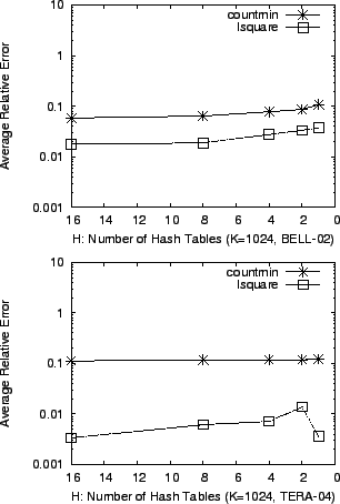
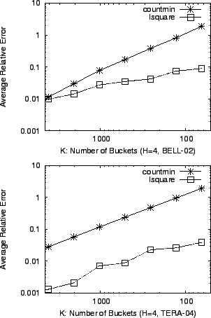
We now evaluate the accuracy of countmin and lsquare under the constraint of limited memory. Since a sketch is usually located within an expensive memory SRAM for high-speed traffic monitoring, it is desirable to have accurate point estimates even if we reduce the size of the sketch.

First, we fix the number of buckets in a hash table $K$ to be $1024$ and vary the number of hash tables $H$. Next, we vary $K$ with fixed $H=4$. In Figure 5 and 6, we calculate the average error of the two methods for each sketch configuration. We can see clearly that the accuracy of lsquare degrades gracefully as the sketch gets smaller, whereas countmin gives inaccurate estimates in memory-limited situations.

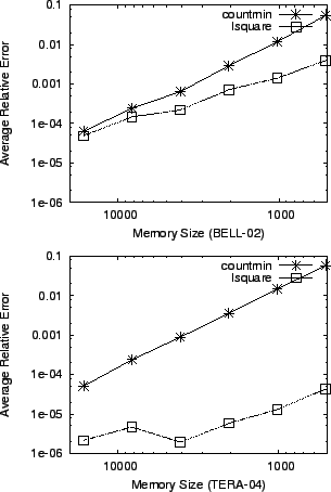
To make the experiment more reliable regardless of the sketch configuration, we find the optimal combination for countmin in the given memory size after trying various combinations of $H$ and $K$. Within the configuration where countmin shows the best accuracy, we evaluate the accuracy of lsquare. Once again, we observe better accuracy of the proposed method (Figure 7).

4.5 Time Performance

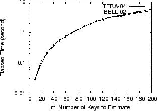
We have implemented our lsquare method in Matlab. The most time-consuming process in our method is solving the linear system $A \mathbf{x}= \mathbf{b}$. We make a preliminary evaluation regarding the time performance of our implementation using a Pentium3-733MHz machine with 128 MBytes memory, operated by Linux Debian 3.0. In this experiment, we use a fixed sketch configuration (H=4, K=1024) and vary the number of heavy hitters we want to estimate. The results in Figure 8 show that the linear program solver can compute point estimations of 100 heavy hitters in about 2 seconds in the given configuration. We note that our current Matlab implementation has not been fully optimized and there is considerable room for further speedup. For example, we can replace the pseudoinverse function pinv with an iterative least-squares solver such as lsqr to take advantage of the sparsity of matrix $A$.

Figure 8: $K=1024$, $H=4$: This graph shows the elapsed time to execute the Linear System Solver with various numbers of heavy hitters.

5 Conclusion and Future Work

In this paper, we propose a new approach for point estimation on sketches. Using extensive experiments with real Internet data sets, we show that the proposed method lsquare is much more accurate than the best existing method countmin. lsquare achieves good reconstruction accuracy for both heavy and light hitters, at the expense of modest computation. Moreover, we have shown that the accuracy of lsquare degrades gracefully as memory decreases. To achieve accuracy comparable to countmin, lsquare in general requires much less memory.

This paper represents an early example on how traditional statistical inference techniques can be applied in the data stream context to infer characteristics of the input stream. Existing research on data stream computation so far has mainly focused on developing techniques that provide provable worst-case accuracy guarantees. Statistical inference techniques in contrast often pay more attention to properties like likelihood, unbiasedness, estimation variance etc. While these inference techniques may not provide any worst-case accuracy guarantees, they often perform very well on practical problems. In our future work, we plan to further explore how statistical inference techniques can be applied to data stream computation.

Bibliography

1

N. Alon, Y. Matias, and M. Szegedy.
The space complexity of approximating the frequency moments.
Journal of Computer and System Sciences, 58(1):137-147, 1999.

2

Bell Labs I data set, 2002.
https://pma.nlanr.net/Traces/long/bell1.html.

3

M. Charikar, K. Chen, and M. Farach-Colton.
Finding frequent items in data streams.
In Proceedings of ICALP '2002, pages 693-703, 2002.
https://www.cs.princeton.edu/~moses/papers/frequent.ps.

4

G. Cormode and S. Muthukrishnan.
What's hot and what's not: Tracking most frequent items dynamically.
In Proceedings of ACM PODC '2003, July 2003.

5

G. Cormode and S. Muthukrishnan.
An improved data stream summary: The count-min sketch and its applications.
Proceedings of Latin American Theoretical Informatics (LATIN), pages 29-38, 2004.

6

C. Estan and G. Varghese.
New directions in traffic measurement and accounting.
Proceedings of ACM SIGCOMM, 2002.

7

P. Gibbons and Y. Matias.
Synopsis structures for massive data sets.
DIMACS Series in Discrete Mathematics and Theoretical Computer Science, 1999.

8

B. Krishnamurthy, S. Sen, Y. Zhang, and Y. Chen.
Sketch-based change detection: Methods, evaluation, and applications.
Proceedings of ACM SIGCOMM Internet Measurement Conference, 2003.

9

A. Kumar, M. Sung, J. Xu, and J. Wang.
Data streaming algorithms for efficient and accurate estimation of flow distribution.
Proceedings of ACM Sigmetrics/Performance, 2004.

10

E. H. Moore.
On the reciprocal of the general algebraic matrix.
Bulletin of the American Mathematical Society, 26:394-395, 1920.

11

S. Muthukrishnan.
Data streams: Algorithms and applications, 2003.
Manuscript based on invited talk from 14th SODA. Available from https://www.cs.rutgers.edu/~muthu/stream-1-1.ps.

12

NLANR.
https://www.nlanr.net/.

13

R. Penrose.
A generalized inverse of matrices.
Mathematical Proceedings of the Cambridge Philosophical Society, 51:406-412, 1955.

14

R. Schweller, A. Gupta, Y. Chen, and E. Parsons.
Reversible sketches for efficient and accurate change detection over network data streams.
Proceedings of ACM SIGCOMM Internet Measurement Conference, pages 207-212, 2004.

15

Teragrid-I 10GigE trace, 2004.
https://pma.nlanr.net/Special/tera1.html.

About this document ...

Improving Sketch Reconstruction Accuracy
Using Linear Least Squares Method

This document was generated using the LaTeX2HTML translator Version 2002-2-1 (1.70)

Copyright © 1993, 1994, 1995, 1996, Nikos Drakos, Computer Based Learning Unit, University of Leeds.
Copyright © 1997, 1998, 1999, Ross Moore, Mathematics Department, Macquarie University, Sydney.

The command line arguments were:
latex2html -split 0 -show_section_numbers -local_icons -image_type gif paper.tex

The translation was initiated by Yin Zhang on 2005-08-09