|
IMC '05 Paper
[IMC '05 Technical Program]
Exploiting Underlying Structure for Detailed
Reconstruction of an Internet-scale Event
Abhishek Kumar
Georgia Institute of Technology
akumar@cc.gatech.edu
Vern Paxson
ICSI
vern@icir.org
Nicholas Weaver
ICSI
nweaver@icsi.berkeley.edu
Abstract
Network ``telescopes'' that record packets sent to
unused blocks of Internet address space have emerged as an important
tool for observing Internet-scale events such as the spread of worms and
the backscatter from flooding attacks that use spoofed source addresses.
Current telescope analyses produce detailed tabulations of packet rates,
victim population, and evolution over time. While such cataloging is a
crucial first step in studying the telescope observations,
incorporating an understanding of the underlying processes generating
the observations allows us to construct detailed inferences about the
broader ``universe'' in which the Internet-scale activity occurs,
greatly enriching and deepening the analysis in the process.
In this work we apply such an analysis to the
propagation of the Witty worm, a malicious and well-engineered
worm that when released in March 2004 infected more than 12,000 hosts
worldwide in 75 minutes. We show that by carefully exploiting the
structure of the worm, especially its pseudo-random number generation,
from limited and imperfect telescope data we can with high fidelity:
extract the individual rate at which each infectee injected packets into
the network prior to loss; correct distortions in the telescope
data due to the worm's volume overwhelming the monitor; reveal the
worm's inability to fully reach all of its potential victims; determine
the number of disks attached to each infected machine; compute when each
infectee was last booted, to sub-second accuracy; explore the ``who
infected whom'' infection tree; uncover that the worm specifically
targeted hosts at a US military base; and pinpoint Patient Zero,
the initial point of infection, i.e., the IP address of the system the
attacker used to unleash Witty.
Network
``telescopes'' have recently emerged as important tools for observing
Internet-scale events such as the spread of worms, the ``backscatter''
of responses from victims attacked by a flood of requests with spoofed
source addresses, and incessant ``background radiation'' consisting of
other anomalous traffic [10,14,15]. Telescopes
record packets sent to unused blocks of Internet address space, with
large ones using /8 blocks covering as much as 1/256 of the total
address space. During network-wide anomalous events, such as the
propagation of a worm, telescopes can collect a small yet significant
slice of the worm's entire traffic. Previously, such logs of worm
activity have been used to infer aggregate properties, such as the
worm's infection rate (number of infected systems), the total scanning
rate (number of worm copies sent per second), and the evolution of these
quantities over time.
The fundamental
premise of our work is that by carefully considering the underlying
structure of the sources sending traffic to a telescope, we can extract
a much more detailed reconstruction of such events. To this end, we
analyze telescope observations of the Witty worm, a malicious and
well-engineered ([21]
analyzes what Witty's design implies about its author.) worm that spread
worldwide in March 2004 in 75 minutes. We show that it is possible to
reverse-engineer the state of each worm infectee's Pseudo-Random Number
Generator (PRNG), which then allows us to recover the full set of
actions undertaken by the worm. This process is greatly complicated by
the worm's use of periodic reseeding of its PRNG, but we show it
is possible to determine the new seeds, and in the process uncover
detailed information about the individual hosts, including access
bandwidth, up-time, and the number of physical drives attached. Our
analysis also enables inferences about the network, such as shared
bottlenecks and the presence or absence of losses on the path from
infectees to the telescope. In addition, we uncover details unique to
the propagation of the Witty worm: its failure to scan about 10% of the
IP address space, the fact that it initially targeted a US military
base, and the identity of Patient Zero -- the host the worm's
author used to release the worm.
Our analysis
reveals systematic distortions in the data collected at telescopes and
provides a means to correct this distortion, leading to more accurate
estimates of quantities such as the worm's aggregate scan rate during
its spread. It also identifies consequences of the specific topological
placement of telescopes. In addition, detailed data about hitherto
unmeasured quantities that emerges from our analysis holds promise to
aid future worm simulations achieve a degree of realism well beyond
today's abstract models. The techniques developed in our study, while
specific to the Witty worm, highlight the power of such analysis, and
provide a template for future analysis of similar events.
We organize the
paper as follows. § 2 presents background
material: the operation of network telescopes and related work, the
functionality of Witty, and the structure of linear-congruential PRNGs.
In § 3 we provide a roadmap to the subsequent
analysis. We discuss how to reverse-engineer Witty's PRNG in § 4, and then use this to estimate access
bandwidth and telescope measurement distortions in § 5.
§ 6 presents a technique for extracting the
seeds used by individual infectees upon reseeding their PRNGs, enabling
measurements of each infectee's system time and number of attached
disks. This section also discusses our exploration of the possible
infector-infectee relationships. We discuss broader consequences of our
study in § 7 and conclude in § 8.
2 Background
Network
Telescopes and Related Work. Network
telescopes operate by monitoring unused or mostly-unused portions of the
routed Internet address space, with the largest able to record traffic
sent to /8 address blocks (16.7M addresses) [10,22]. The telescope consists
of a monitoring machine that passively records all packets headed to any
of the addresses in the block. Since there are few or no actual machines
using these addresses, traffic headed there is generally anomalous, and
often malicious, in nature. Examples of traffic observed at network
telescopes include port and address scans, ``backscatter'' from flooding
attacks, misconfigurations, and the worm packets that are of immediate
interest to this work.
The first major
study performed using a network telescope was the analysis of
backscatter by Moore et al. [14]. This
study assessed the prevalence and characteristics of spoofed-source
denial-of-service (DoS) attacks and the characteristics of the victim
machines. The work built on the observation that most DoS tools that
spoof source addresses pick addresses without a bias towards or against
the telescope's observational range. The study also inferred victim
behavior by noting that the response to spoofed packets will depend on
the state of the victim, particularly whether there are services running
on the targeted ports.
Telescopes have
been the primary tool for understanding the Internet-wide spread of
previous worms, beginning with Code Red [2,20]. Since, for a random-scanning
worm, the worm is as likely to contact a telescope address as a normal
address, we can extrapolate from the telescope data to compute the
worm's aggregate scanning rate as it spreads. In addition, from
telescope data we can see which systems were infected, thus estimate the
average worm scanning rate. For high-volume sources, we can also
estimate a source's effective bandwidth based on the rate at which its
packets arrive and adjusting for the telescope's ``gathering power''
(portion of entire space monitored).
A variation is the distributed
telescope, which monitors a collection of disparate address ranges
to create an overall picture [1,4]. Although some phenomena
[6,2]) scan uniformly,
others either have biases in their address selection [11,12] or simply exclude some
address ranges entirely [5,16]. Using a distributed
telescope allows more opportunity to observe nonuniform phenomenon, and
also reveals that, even correcting for ``local preference'' biases
present in some forms of randomized scanning, different telescopes
observe quantitatively different phenomena [4].
The biggest
limitation of telescopes is their passive nature, which often limits the
information we can gather. One solution useful for some studies has
been active telescopes: changing the telescope logic to either
reply with SYN-ACKs to TCP SYNs in order to capture the resulting
traffic [4], or
implementing a more complex state machine [15] that emulates
part of the protocol. These telescopes can disambiguate scans from
different worms that target the same ports by observing subsequent
transactions.
In this work we
take a different approach for enhancing the results of telescope
measurements: augmenting traces from a telescope with a detailed
analysis of the structure of the sources sending the packets. One key
insight is that the PRNG used to construct ``random'' addresses for a
worm can leak the internal state of the PRNG. By combining the
telescope data with our knowledge of the PRNG, we can then determine the
internal state for each copy of the worm and see how this state evolves
over time.
While there have
been numerous studies of Internet worms, these have either focused on
detailed analysis of the worm's exact workings, beginning with analysis
of the 1988 Morris Worm [7,19], or with aggregate
propagation dynamics [23,11,18,20,13]. In contrast, our
analysis aims to develop a detailed understanding of the individual
infected hosts and how they interacted with the network.
Datasets. We
used traces from two telescopes, operated by CAIDA [10] and the University of
Wisconsin [22]. Both
telescopes monitor /8 blocks of IP addresses. Since each /8 contains
1/256 of all valid IPv4 addresses, these telescopes see an equivalent
fraction of scan traffic addressed to random destinations picked
uniformly from the 32-bit IP address space. The CAIDA telescope logs
every packet it receives, while the Wisconsin telescope samples the
received packets at the rate of 1/10. The CAIDA trace [17] begins at 04:45 AM
UTC, running for 75 minutes and totaling 45.5M packets. The Wisconsin
trace runs from 04:45 AM UTC for 75 minutes, totaling 4.1M packets.
Functionality
of the Witty worm. As chronicled by Shannon
and Moore [18], an
Internet worm was released on Friday March 19, 2004 at approximately
8:45 PM PST (4:45 AM UTC, March 20). Its payload contained the phrase ``(^.^)
insert witty message here (^.^)'' so it came to be
known as the Witty worm. The worm targeted a buffer overflow
vulnerability in several Internet Security Systems (ISS) network
security products.
Figure 1: Functionality of the
Witty worm
 |
The vulnerability
exploited was a stack-based overflow in the ICQ analyzer of these
security products. When they received an ICQ packet, defined as any UDP
packet with source port 4000 and the appropriate ICQ headers,
they copied the packet into a fixed-sized buffer on the stack in
preparation for further analysis. The products executed this code path
regardless of whether a server was listening for packets on the
particular UDP destination port. In addition, some products could become
infected while they passively monitored network links
promiscuously, because they would attempt to analyze ICQ packets seen on
the link even though they were not addressed to the local host.
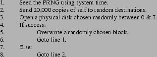
Figure 1 shows a high-level description of the
functionality of the Witty worm, as revealed by a disassembly [9]. The worm is
quite compact, fitting in the first 675 bytes of a single UDP packet.
Upon infecting a host, the worm first seeds its random number generator
with the system time on the infected machine and then sends 20,000
copies of itself to random destinations. (These packets have a randomly
selected destination port and a randomized amount of additional
padding, but keep the source port fixed.) After sending the 20,000
packets, the worm uses a three-bit random number to pick a disk via the
open system call. If the call returns successfully, the worm overwrites
a random block on the chosen disk, reseeds its PRNG, and goes back to
sending 20,000 copies of itself. Otherwise, the worm jumps directly to
the send loop, continuing for another 20,000 copies, without
reseeding its PRNG.
The LC PRNG. The Witty worm used a simple feedback-based
pseudo-random number generator (PRNG) of the form known as linear
congruential (LC):
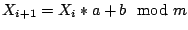 |
(1) |
For a given  , picking effective values of , picking effective values of  and and  requires care lest the resulting sequences lack basic
properties such as uniformity. One common parameterization is: requires care lest the resulting sequences lack basic
properties such as uniformity. One common parameterization is: 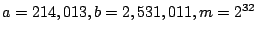 . .
With the above
values of  , the LC PRNG generates a permutation of
all the integers in , the LC PRNG generates a permutation of
all the integers in ![$ \left[0,m-1\right]$](img10.png) . A key point then is that with knowledge
of any . A key point then is that with knowledge
of any  , all subsequent pseudo-random numbers in
the sequence can be generated by repeatedly applying Eqn 1.
It is also possible to invert Eqn 1 to compute if the value of , all subsequent pseudo-random numbers in
the sequence can be generated by repeatedly applying Eqn 1.
It is also possible to invert Eqn 1 to compute if the value of  is known: is known:
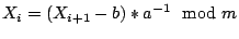 |
(2) |
where, for  , , 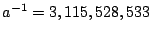 . .
Eqns 1
and 2 provide us with the machinery to generate
the entire sequence of random numbers as generated by an LC PRNG, either
forwards or backwards, from any arbitrary starting point on the
sequence. Thus, if we can extract any , we can
compute any other  , given , given  . However, it is
important to note that most uses of pseudo-random numbers, including
Witty's, do not directly expose any , but rather
extract a subset of 's bits and intermingle them
with bits from additionally generated pseudo-random numbers, as
detailed below. . However, it is
important to note that most uses of pseudo-random numbers, including
Witty's, do not directly expose any , but rather
extract a subset of 's bits and intermingle them
with bits from additionally generated pseudo-random numbers, as
detailed below.
3 Overview of our analysis
The first step in
our analysis, covered in § 4, is to develop a
way to uncover the state of an infectee's PRNG. It turns out that we
can do so from the observation of just a single packet sent by the
infectee and seen at the telescope. (Note, however, that if recovering
the state required observing consecutive packets, we would likely often
still be able to do so: while the telescopes record on average only one
in 256 packets transmitted by an infectee, occasionally -- i.e., roughly
one time out of 256 -- they will happen to record consecutive packets.)
An interesting fact
revealed by careful inspection of the use of pseudo-random numbers by
the Witty worm is that the worm does not manage to scan the entire
32-bit address space of the Internet, in spite of using a correct
implementation of the PRNG. This analysis also reveals the identity of a
special host that very likely was used to start the worm.
Once we have the
crucial ability to determine the state of an infectee's PRNG, we can use
this state to reproduce the worm's exact actions, which then allows us
to compare the resulting generated packets with the actual packets seen
at the telescope. This comparison yields a wealth of information about
the host generating the packets and the network the packets traversed.
First, we can determine the access bandwidth of the infectee,
i.e., the capacity of the link to which its network interface connects.
In addition, given this estimate we can explore significant flaws in
the telescope observations, namely packet losses due to the finite
bandwidth of the telescope's inbound link. These losses cause a
systematic underestimation of infectee scan rates, but we design a
mechanism to correct for this bias by calibrating against our
measurements of the access bandwidth. We also highlight the impact of
network location of telescopes on the observations they collect (§ 5).
We next observe
that choosing a random disk (line 3 of Figure 1)
consumes another pseudo-random number in addition to those consumed by
each transmitted packet. Observing such a discontinuity in the sequence
of random numbers in packets from an infectee flags an attempted disk
write and a potential reseeding of the infectee's PRNG. In § 6 we develop a detailed mechanism to detect the
value of the seed at each such reseeding. As the seed at line 1 of Fig. 1 is set to the system time in msec since boot up,
this mechanism allows us to estimate the boot time of individual
infectees just by looking at the sequence of occasional packets received
at the telescope. Once we know the PRNG's seed, we can precisely
determine the random numbers it generates to synthesize the next 20,000
packets, and also the three-bit random number it uses next time to pick
a physical disk to open. We can additionally deduce the success or
failure of this open system call by whether the PRNG state for
subsequent packets from the same infectee follow in the same series or
not. Thus, this analysis reveals the number of physical disks on the
infectee.
Lastly, knowledge
of the seeds also provides access to the complete list of packets sent
by the infectee. This allows us to infer infector-infectee relationships
during the worm's propagation.
4 Analysis of Witty's PRNG
Figure 2: Pseudocode of the Witty
worm
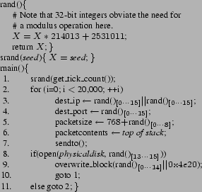 |
The first step in
our analysis is to examine a disassembly of the binary code of the Witty
worm [9].
Security researchers typically publish such disassemblies immediately
after the release of a worm in an attempt to understand the worm's
behavior and devise suitable countermeasures. Figure 2
shows the detailed pseudocode of the Witty worm as derived from one such
disassembly [9].
The rand() function implements the Linear Congruential PRNG as discussed
in § 2. In the rest of this section, we use
the knowledge of the pseudocode to develop a technique for deducing the
state of the PRNG at an infectee from any single packet sent by
it. We also describe how as a consequence of the specific manner in
which Witty uses the pseudo-random numbers, the worm fails to scan the
entire IP address space, and also reveals the identity of Patient
Zero.
Breaking the
state of the PRNG at the infectee. The
Witty worm constructs ``random'' destination IP addresses by
concatenating the top 16 bits of two consecutive pseudo random numbers
generated by its PRNG. In our notation, ![$ X_{[0\cdots 15]}$](img19.png) represents the top 16 bits of the 32 bit
number represents the top 16 bits of the 32 bit
number  , with bit 0 being the most significant.
The destination port number is constructed by taking the top 16 bits of
the next (third) random number. The packet size (The main body of the
Witty worm, including the initial pad required to cause the buffer
overflow, fits in 675 bytes. However, the worm picks a larger
packet-size, as shown in line 5 of Fig. 2, and
pads the tail of the packet with whatever is on the stack, presumably to
complicate the use of static filtering to block the contagion.) itself is
chosen by adding the top 9 bits of a fourth random number to 768. Thus,
each packet sent by the Witty worm contains bits from four consecutive
random numbers, corresponding to lines 3,4 and 5 in Fig. 2. If all 32 bits of any of these numbers were
known, it would completely specify the state of the PRNG. But since only
some of the bits from each of these numbers is known, we need to design
a mechanism to retrieve all 32 bits of one of these numbers from the
partial information contained in each packet. , with bit 0 being the most significant.
The destination port number is constructed by taking the top 16 bits of
the next (third) random number. The packet size (The main body of the
Witty worm, including the initial pad required to cause the buffer
overflow, fits in 675 bytes. However, the worm picks a larger
packet-size, as shown in line 5 of Fig. 2, and
pads the tail of the packet with whatever is on the stack, presumably to
complicate the use of static filtering to block the contagion.) itself is
chosen by adding the top 9 bits of a fourth random number to 768. Thus,
each packet sent by the Witty worm contains bits from four consecutive
random numbers, corresponding to lines 3,4 and 5 in Fig. 2. If all 32 bits of any of these numbers were
known, it would completely specify the state of the PRNG. But since only
some of the bits from each of these numbers is known, we need to design
a mechanism to retrieve all 32 bits of one of these numbers from the
partial information contained in each packet.
To do so, if the
first call to rand() returns , then:
where  is the concatenation
operation. Now, we know that and are related by Eqn 1, and so are and is the concatenation
operation. Now, we know that and are related by Eqn 1, and so are and  . Furthermore, there
are only 65,536 ( . Furthermore, there
are only 65,536 ( ) possibilities for
the lower 16 bits of , and only one of
them is such that when used with ) possibilities for
the lower 16 bits of , and only one of
them is such that when used with ![$ X_{i,[0\cdots 15]}$](img29.png) (available from the
packet) the next two numbers generated by Eqn 1 have the same top
16 bits as (available from the
packet) the next two numbers generated by Eqn 1 have the same top
16 bits as ![$ X_{i+1,[0\cdots
15]}$](img30.png) and and ![$ X_{i+2,[0\cdots 15]}$](img31.png) , which are also
observed in the received packet. In other words, there is only one
16-bit number , which are also
observed in the received packet. In other words, there is only one
16-bit number  that satisfies the
following two equations simultaneously:
For each of the possible values of , verifying the first
equality takes one addition and one multiplication. (Since that satisfies the
following two equations simultaneously:
For each of the possible values of , verifying the first
equality takes one addition and one multiplication. (Since  , the modulo
operation is implemented implicitly by the use of 32 bit registers and
disregarding their overflow during arithmetic operations.) Thus trying
all possibilities is
fairly inexpensive. For the small number of possible values of that satisfy the
first equation, we try the second equation, and the value , the modulo
operation is implemented implicitly by the use of 32 bit registers and
disregarding their overflow during arithmetic operations.) Thus trying
all possibilities is
fairly inexpensive. For the small number of possible values of that satisfy the
first equation, we try the second equation, and the value  that satisfies both
the equations gives us the lower sixteen bits of (i.e., that satisfies both
the equations gives us the lower sixteen bits of (i.e., ![$ X_{i,[16\cdots 31]}=Y^*$](img37.png) ). In our
experiments, we found that on the average about two of the possible values
satisfy the first equation, but there was always a unique value of that satisfied both
the equations. ). In our
experiments, we found that on the average about two of the possible values
satisfy the first equation, but there was always a unique value of that satisfied both
the equations.
Why Witty fails
to scan the entire address space. The
first and somewhat surprising outcome from investigating how Witty
constructs random destination addresses is the observation that Witty
fails to scan the entire IP address space. This means that, while Witty
spread at a very high speed (infecting 12,000 hosts in 75 minutes), due
to a subtle error in its use of pseudo-random numbers about 10% of
vulnerable hosts were never infected with the worm.
To understand this
flaw in full detail, we first visit the motivation for the use of only
the top 16 bits of the 32 bit results returned by Witty's LC PRNG. This
was recommended by Knuth [8],
who showed that the high order bits are ``more random'' than the lower
order bits returned by the LC PRNG. Indeed, for this very reason,
several implementations of the rand() function, including the default C
library of Windows and SunOS, return a 15 bit number, even though their
underlying LC PRNG uses the same parameters as the Witty worm and
produces 32 bit numbers.
However, this
advice was taken out of context by the author of the Witty worm. Knuth's
advice applies when uniform randomness is the desired property,
and is valid only when a small number of random bits are needed. For a
worm trying to maximize the number of infected hosts, one reason for
using random numbers while selecting destinations is to avoid detection
by intrusion detection systems that readily detect sequential scans. A
second reason is to maintain independence between the portions of the
address-space scanned by individual infectees. Neither of these reasons
actually requires the kind of ``good randomness'' provided by following
Knuth's advice of picking only the higher order bits.
As discussed in § 2, for specific values of the parameters  and , the LC PRNG is a permutation PRNG
that generates a permutation of all integers in the range 0 to and , the LC PRNG is a permutation PRNG
that generates a permutation of all integers in the range 0 to  . By the above definition, if the Witty worm were to use
the entire 32 bits of a single output of its LC PRNG as a destination
address, it would eventually generate each possible 32-bit number, hence
successfully scanning the entire IP address space. (This would also of
course make it trivial to recover the PRNG state.) However, the worm's
author chose to use the concatenation of the top 16 bits of two
consecutive random numbers from its PRNG. With this action, the
guarantee that each possible 32-bit number will be generated is lost. In
other words, there is no certainty that the set of 32-bit numbers
generated in this manner will include all integers in the set . By the above definition, if the Witty worm were to use
the entire 32 bits of a single output of its LC PRNG as a destination
address, it would eventually generate each possible 32-bit number, hence
successfully scanning the entire IP address space. (This would also of
course make it trivial to recover the PRNG state.) However, the worm's
author chose to use the concatenation of the top 16 bits of two
consecutive random numbers from its PRNG. With this action, the
guarantee that each possible 32-bit number will be generated is lost. In
other words, there is no certainty that the set of 32-bit numbers
generated in this manner will include all integers in the set ![$ [0,2^{32}-1]$](img40.png) . .
We enumerated
Witty's entire ``orbit'' and found that there are 431,554,560 32-bit
numbers that can never be generated. This corresponds to 10.05% of the
IP address space that was never scanned by Witty. On further
investigation, we found these unscanned addresses to be fairly uniformly
distributed over the 32-bit address space of IPv4. Hence, it is
reasonable to assume that approximately the same fraction of the populated
IP address space was missed by Witty. In other words, even though the
portions of IP address space that are actually used (populated) are
highly clustered, because the addresses that Witty misses are uniformly
distributed over the space of 32-bit integers, it missed roughly the
same fraction of address among the set of IP addresses in actual use.
Observing that
Witty does not visit some addresses at all, one might ask whether it
visits some addresses more frequently than others. Stated more formally,
given that the period of Witty's PRNG is  , it must
generate unique , it must
generate unique  pairs, from which it constructs
32-bit destination IP addresses. Since this set of
addresses does not contain the 431,554,560 addresses missed by Witty, it
must contain some repetitions. What is the nature of these repetitions?
Interestingly, there are exactly 431,554,560 other 32-bit numbers
that occur twice in this set, and no 32-bit numbers that occur three or
more times. This is surprising because, in general, in lieu of the
431,554,560 missed numbers, one would expect some number to be visited
twice, others to be visited thrice and so on. However, the peculiar
structure of the sequence generated by the LC PRNG with specific
parameter values created the situation that exactly the same number of
other addresses were visited twice and none were visited more
frequently. pairs, from which it constructs
32-bit destination IP addresses. Since this set of
addresses does not contain the 431,554,560 addresses missed by Witty, it
must contain some repetitions. What is the nature of these repetitions?
Interestingly, there are exactly 431,554,560 other 32-bit numbers
that occur twice in this set, and no 32-bit numbers that occur three or
more times. This is surprising because, in general, in lieu of the
431,554,560 missed numbers, one would expect some number to be visited
twice, others to be visited thrice and so on. However, the peculiar
structure of the sequence generated by the LC PRNG with specific
parameter values created the situation that exactly the same number of
other addresses were visited twice and none were visited more
frequently.
Figure 3: Growth curves for
victims whose addresses were scanned once per orbit, twice per orbit, or
not at all.
|
|
During the first 75
minutes of the release of the Witty worm, the CAIDA telescope saw 12,451
unique IP addresses as infected. Following the above discussion, we
classified these addresses into three classes. There were 10,638
(85.4%) addresses that were scanned just once in an orbit, i.e.,
addresses that experienced a normal scan rate. Another 1,409 addresses
(11.3%) were scanned twice in an orbit, hence experiencing twice the
normal growth rate. A third class of 404 (3.2%) addresses belonged to
the set of addresses never scanned by the worm. At first blush
one might wonder how these latter could possibly appear, but we can
explain their presence as reflecting inclusion in an initial ``hit
list'' (see below), operating in promiscuous mode, or aliasing due to
multi-homing, NAT or DHCP.
Figure 3 compares the growth curves for the three
classes of addresses. Notice how the worm spreads faster among the
population of machines that experience double the normal scan rate.
1,000 sec from its release, Witty had infected half of the
doubly-scanned addresses that it would infect in the first 75 min. On
the other hand, in the normally-scanned population, it had only managed
to infect about a third of the total victims that it would infect in
75 min. Later in the hour, the curve for the doubly-scanned addresses is
flatter than that for the normally-scanned ones, indicating that most of
the victims in the doubly-scanned population were already infected at
that point.
The curve for
infectees whose source address was never scanned by Witty is
particularly interesting. Twelve of the never-scanned systems appear in
the first 10 seconds of the worm's propagation, very strongly suggesting
that they are part of an initial hit-list. This explains the early jump
in the plot: it's not that such machines are overrepresented in the
hit-list, rather they are underrepresented in the total infected
population, making the hit-list propagation more significant for this
population.
Another class of
never-scanned infectees are those passively monitoring a network link.
Because these operate in promiscuous mode, their ``cross section'' for
becoming infected is magnified by the address range routed over the
link. On average, these then will become infected much more rapidly than
normal over even doubly-scanned hosts. We speculate that these
infectees constitute the remainder of the early rise in the appearance
of never-scanned systems. Later, the growth rate of the never-scanned
systems substantially slows, lagging even the single-scanned addresses.
Likely these remaining systems reflect infrequent aliasing due to
multihoming, NAT, or DHCP.
Identifying
Patient Zero. Along with ``Can all addresses
be reached by scans?'', another question to ask is ``Do all sources
indeed travel on the PRNG orbit?'' Surprisingly, the answer is No.
There is a single Witty source that consistently fails to follow the
orbit. Further inspection reveals that the source (i) always
generates addresses of the form  rather than rather than  , (ii) does not randomize the packet size, and (iii)
is present near the very beginning of the trace, but not before the worm
itself begins propagating. That the source fails to follow the orbit
clearly indicates that it is running different code than do all
the others; that it does not appear prior to the worm's onset indicates
that it is not a background scanner from earlier testing or probing
(indeed, it sends valid Witty packets which could trigger an infection);
and that it sends to sources of a limited form suggests a bug in its
structure that went unnoticed due to a lack of testing of this
particular Witty variant. , (ii) does not randomize the packet size, and (iii)
is present near the very beginning of the trace, but not before the worm
itself begins propagating. That the source fails to follow the orbit
clearly indicates that it is running different code than do all
the others; that it does not appear prior to the worm's onset indicates
that it is not a background scanner from earlier testing or probing
(indeed, it sends valid Witty packets which could trigger an infection);
and that it sends to sources of a limited form suggests a bug in its
structure that went unnoticed due to a lack of testing of this
particular Witty variant.
We argue that these
peculiarities add up to a strong likelihood that this unique host
reflects Patient Zero, the system used by the attacker to seed
the worm initially. Patient Zero was not running the complete Witty worm
but rather a (not fully tested) tool used to launch the worm. To our
knowledge, this represents the first time that Patient Zero has been
identified for a major worm outbreak. (The only related case of which we
are aware was the Melissa email virus [3], where the author posted
the virus to USENET as a means of initially spreading his malcode, and
was traced via USENET headers.) We have conveyed the host's IP address
(which corresponds to a European retail ISP) to law enforcement.
If all Patient Zero
did was send packets of the form as we
observed, then the worm would not have spread, as we detected no
infectees with such addresses. However, as developed both above in
discussing Figure 3 and later in § 6, the evidence is compelling that Patient Zero
first worked through a ``hit list'' of known-vulnerable hosts before
settling into its ineffective scanning pattern.
5 Bandwidth measurements
An important use of
network telescopes lies in inferring the scanning rate of a worm by
extrapolating from the observed packets rates from individual sources.
In this section, we develop a technique based on our analysis of Witty's
PRNG to estimate the access bandwidth of individual infectees. We then
identify an obvious source of systematic error in extrapolation based
techniques, namely the bottleneck at the telescope's inbound link, and
suggest a solution to correct this error.
Estimating
Infectee Access Bandwidth. The access bandwidth of the population of
infected machines is an important variable in the dynamics of the spread
of a worm. Using the ability to deduce the state of the PRNG at an
infectee, we can infer this quantity, as follows. The Witty worm uses
the sendto system call, which is a blocking system call by
default in Windows: the call will not return till the packet has been
successfully written to the buffer of the network interface. Thus, no
worm packets are dropped either in the kernel or in the buffer of the
network interface. But the network interface can clear out its buffer at
most at its transmission speed. Thus, the use of blocking system calls
indirectly clocks the rate of packet generation of the Witty worm to
match the maximum transmission bandwidth of the network interface on
the infectee.
We estimate the
access bandwidth of an infectee as follows. Let  and and  be two packets from the same infectee, received at the
telescope at time be two packets from the same infectee, received at the
telescope at time  and and  respectively.
Using the mechanism developed in § 4
we can deduce and respectively.
Using the mechanism developed in § 4
we can deduce and  , the state of
the PRNG at the sender when the two respective packets were sent. Now,
we can simulate the LC PRNG with an initial state of and
repeatedly apply Eqn 1 till the state advances to . The number of times Eqn 1 is applied
to get from to is the value of , the state of
the PRNG at the sender when the two respective packets were sent. Now,
we can simulate the LC PRNG with an initial state of and
repeatedly apply Eqn 1 till the state advances to . The number of times Eqn 1 is applied
to get from to is the value of  . Since it takes 4 cranks of the PRNG to construct each
packet (lines 3-5, in Fig. 2), the total number
of packets between and is . Since it takes 4 cranks of the PRNG to construct each
packet (lines 3-5, in Fig. 2), the total number
of packets between and is  . Thus the access bandwidth of the infectee is
approximately . Thus the access bandwidth of the infectee is
approximately 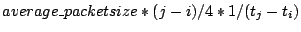 . While we can
compute it more precisely, since reproducing the PRNG sequence lets us
extract the exact size of each intervening packet sent, for convenience
we will often use the average payload size (1070 bytes including UDP, IP
and Ethernet headers). Thus, the transmission rate can be computed as . While we can
compute it more precisely, since reproducing the PRNG sequence lets us
extract the exact size of each intervening packet sent, for convenience
we will often use the average payload size (1070 bytes including UDP, IP
and Ethernet headers). Thus, the transmission rate can be computed as 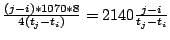 bits per second.
Figure 4: Access bandwidth of
Witty infectees estimated using our technique.
|
|
Figure 4 shows the estimates of access bandwidth of
infectees (We ignore infectees that contributed  20
packets.) that appeared at the CAIDA telescope from 05:01 AM to 06:01 AM
UTC (i.e., starting about 15 min after the worm's release). The 20
packets.) that appeared at the CAIDA telescope from 05:01 AM to 06:01 AM
UTC (i.e., starting about 15 min after the worm's release). The  -axis shows the estimated access bandwidth in bps on log
scale, and the -axis shows the estimated access bandwidth in bps on log
scale, and the  -axis shows the rank of each infectee in
increasing order. It is notable in the figure that about 25% of the
infectees have an access bandwidth of 10 Mbps while about 50% have a
bandwidth of 100 Mbps. This corresponds well with the popular
workstation configurations connected to enterprise LANs (a likely
description of a machine running the ISS software vulnerable to Witty),
or to home machines that include an Ethernet segment connecting to a
cable or DSL modem. -axis shows the rank of each infectee in
increasing order. It is notable in the figure that about 25% of the
infectees have an access bandwidth of 10 Mbps while about 50% have a
bandwidth of 100 Mbps. This corresponds well with the popular
workstation configurations connected to enterprise LANs (a likely
description of a machine running the ISS software vulnerable to Witty),
or to home machines that include an Ethernet segment connecting to a
cable or DSL modem.
Figure 5: Comparison of estimated
access bandwidth using data from two telescopes.
|
|
We use the second
set of observations, collected independently at the Wisconsin telescope
(located far from the CAIDA telescope), to test the accuracy of our
estimation, as shown in Figure 5. Each point
in the scatter plot represents a source observed in both datasets, with
its and coordinates
reflecting the estimates from the Wisconsin and CAIDA observations,
respectively. Most points are located very close to the  line, signifying close agreement. The small number of points (about 1%)
that are significantly far from the line merit
further investigation. We believe these reflect NAT effects invalidating
our inferences concerning the amount of data a ``single'' source sends
during a given interval.
line, signifying close agreement. The small number of points (about 1%)
that are significantly far from the line merit
further investigation. We believe these reflect NAT effects invalidating
our inferences concerning the amount of data a ``single'' source sends
during a given interval.
Extrapolation-based
estimation of effective bandwidth. Previous analyses of telescope
data (e.g., [18]) used a
simple extrapolation-based technique to estimate the bandwidth of the
infectees. The reasoning is that given a telescope captures a /8 address
block, it should see about 1/256 of the worm traffic. Thus, after
computing the packets per second from individual infectees, one can
extrapolate this observation by multiplying by 256 to estimate the total
packets sent by the infectee in the corresponding period. Multiplying
again by the average packet size (1070 bytes) gives the
extrapolation-based estimate of the bandwidth of the infectee. Notice
that this technique is not measuring the access bandwidth of the
infectee, but rather the effective bandwidth, i.e., the rate at
which packets from the infectee are actually delivered across the
network.
Figure 6: Effective bandwidth of
Witty infectees.
|
|
Figure 7: Scatter-plot of
estimated bandwidth using the two techniques.
|
|
Figure 6 shows the estimated bandwidth of the same
population of infectees, computed using the extrapolation technique. The
effective bandwidth so computed is significantly lower than the access
bandwidth of the entire population. To explore this further, we draw a
scatter-plot of the estimates using both techniques in Fig. 7. Each point corresponds to the
PRNG-estimated access bandwidth ( axis) and
extrapolation-based effective bandwidth ( axis). The modes
at 10 and 100 Mbps in Fig. 4 manifest as clusters
of points near the lines  and and  ,
respectively. As expected, all points lie below the diagonal,
indicating that the effective bandwidth never exceeds the access
bandwidth, and is often lower by a significant factor. During infections
of bandwidth-limited worms, i.e., worms such as Witty that send fast
enough to potentially consume all of the infectee's bandwidth, mild to
severe congestion, engendering moderate to significant packet losses, is
likely to occur in various portions of the network. ,
respectively. As expected, all points lie below the diagonal,
indicating that the effective bandwidth never exceeds the access
bandwidth, and is often lower by a significant factor. During infections
of bandwidth-limited worms, i.e., worms such as Witty that send fast
enough to potentially consume all of the infectee's bandwidth, mild to
severe congestion, engendering moderate to significant packet losses, is
likely to occur in various portions of the network.
Another possible
reason for observing diminished effective bandwidth is multiple
infectees sharing a bottleneck, most likely because they reside within
the same subnet and contend for a common uplink. Indeed, this effect is
noticeable at /16 granularity. That is, sources exhibiting very high
loss rates (effective bandwidth 10% of access
bandwidth) are significantly more likely to reside in /16 prefixes that
include other infectees, than are sources with lower loss rates
(effective  50% access). For example, only 20% of the
sources exhibiting high loss reside alone in their own /16, while 50% of
those exhibiting lower loss do. 50% access). For example, only 20% of the
sources exhibiting high loss reside alone in their own /16, while 50% of
those exhibiting lower loss do.
Figure 8: Aggregate worm traffic
in pkts/sec as actually logged at the telescope.
|
|
Telescope
Fidelity. An
important but easy-to-miss feature of Fig. 7
is that the upper envelope of the points is not the line but rather  , which shows up as the upper envelope of the
scatter plot lying parallel to, but slightly below, the diagonal. This
implies either a loss rate of nearly 30% for even the best connected
infectees, or a systematic error in the observations. Further
investigation immediately reveals the cause of the systematic error,
namely congestion on the inbound link of the telescope. Figure 8 plots the packets received during one-second
windows against time from the release of the worm. There is a clear
ramp-up in aggregate packet rate during the initial 800 seconds after
which it settles at approximately 11,000 pkts/sec. For an average packet
size of 1,070 bytes, a rate of 11,000 pkts/sec corresponds to 95 Mbps,
nearly the entire inbound bandwidth of 100 Mbps of the CAIDA telescope
at that time. (We can attribute the missing 5 Mbps to other, ever-present
``background radiation'' that is a constant feature at such telescopes [15].) , which shows up as the upper envelope of the
scatter plot lying parallel to, but slightly below, the diagonal. This
implies either a loss rate of nearly 30% for even the best connected
infectees, or a systematic error in the observations. Further
investigation immediately reveals the cause of the systematic error,
namely congestion on the inbound link of the telescope. Figure 8 plots the packets received during one-second
windows against time from the release of the worm. There is a clear
ramp-up in aggregate packet rate during the initial 800 seconds after
which it settles at approximately 11,000 pkts/sec. For an average packet
size of 1,070 bytes, a rate of 11,000 pkts/sec corresponds to 95 Mbps,
nearly the entire inbound bandwidth of 100 Mbps of the CAIDA telescope
at that time. (We can attribute the missing 5 Mbps to other, ever-present
``background radiation'' that is a constant feature at such telescopes [15].)
Fig. 8 suggests that the telescope may not have
suffered any significant losses in the first 800 seconds of the spread
of the worm. We verified this using a scatter-plot similar to Fig. 7, but only for data collected in the
first 600 seconds of the infection. In that plot, omitted here due to
lack of space, the upper envelope is indeed , indicating
that the best connected infectees were able to send packets unimpeded
across the Internet, as fast as they could generate them.
A key point here is
that our ability to determine access bandwidth allows us to quantify
the 30% distortion (The distortion is not static but evolves with the
spread of the worm. By tracking changes in the slope of the upper
envelope, we can infer the value of the distortion against time
throughout the period of activity of the worm. at the telescope due to
its limited capacity.) In the absence of this fine-grained analysis, we
would have been limited to noting that the telescope saturated, but
without knowing how much we were therefore missing.
Figure 9: Comparison of effective
bandwidth as estimated at the two telescopes.
|
|
Figure 9 shows a scatter-plot of the estimates of
effective bandwidth as estimated from the observations at the two
telescopes. We might expect these to agree, with most points lying close
to the line, other than perhaps for differing
losses due to saturation at the telescopes themselves, for which we can
correct. Instead, we find two major clusters that lie approximately
along  and and  . These lie
parallel to the line due to the logscale on both axes. We
see a smaller third cluster below the line, too.
These clusters indicate systematic divergence in the telescope
observations, and not simply a case of one telescope suffering
more saturation losses than the other, which would result in a single
line either above or below . . These lie
parallel to the line due to the logscale on both axes. We
see a smaller third cluster below the line, too.
These clusters indicate systematic divergence in the telescope
observations, and not simply a case of one telescope suffering
more saturation losses than the other, which would result in a single
line either above or below .
To analyze this
effect, we took all of the sources with an effective bandwidth estimate
from both telescopes of more than 10 Mbps. We resolved each of these to
domain names via reverse DNS lookups, taking the domain of the
responding nameserver if no PTR record existed. We then selected a
representative for each of the unique second-level domains present among
these, totaling 900. Of these, only 29 domains had estimates at the
two telescopes that agreed within 5% after correcting for systematic
telescope loss. For 423 domains, the corrected estimates at CAIDA
exceeded those at Wisconsin by 5% or more, while the remaining 448 had
estimates at Wisconsin that exceeded CAIDA's by 5% or more.
Table 1: Domains with divergent estimates of
effective bandwidth.
CAIDA  Wisc.*1.05 Wisc.*1.05 |
Wisc. CAIDA*1.05 |
| # Domains |
TLD |
# Domains |
TLD |
| 53 |
.edu |
64 |
.net |
| 17 |
.net |
35 |
.com |
| 7 |
.jp |
9 |
.edu |
| 5 |
.nl |
7 |
.cn |
| 5 |
.com |
5 |
.nl |
| 5 |
.ca |
4 |
.ru |
| 3 |
.tw |
3 |
.jp |
| 3 |
.gov |
3 |
.gov |
| 25 |
other |
19 |
other |
|
Table 1 lists the top-level domains for the unique
second-level domains that demonstrated  % divergence
in estimated effective bandwidth. Owing to its connection to
Internet-2, the CAIDA telescope saw packets from .edu with significantly
fewer losses than the Wisconsin telescope, which in turn had a better
reachability from hosts in the .net and .com domains. Clearly,
telescopes are not ``ideal'' devices, with perfectly balanced
connectivity to the rest of the Internet, as implicitly assumed by
extrapolation-based techniques. Rather, what a telescope sees during an
event of large enough volume to saturate high-capacity Internet links
is dictated by its specific location on the Internet topology. This
finding complements that of [4],
which found that the (low-volume) background radiation seen at
different telescopes likewise varies significantly with location, beyond
just the bias of some malware to prefer nearby addresses when scanning. % divergence
in estimated effective bandwidth. Owing to its connection to
Internet-2, the CAIDA telescope saw packets from .edu with significantly
fewer losses than the Wisconsin telescope, which in turn had a better
reachability from hosts in the .net and .com domains. Clearly,
telescopes are not ``ideal'' devices, with perfectly balanced
connectivity to the rest of the Internet, as implicitly assumed by
extrapolation-based techniques. Rather, what a telescope sees during an
event of large enough volume to saturate high-capacity Internet links
is dictated by its specific location on the Internet topology. This
finding complements that of [4],
which found that the (low-volume) background radiation seen at
different telescopes likewise varies significantly with location, beyond
just the bias of some malware to prefer nearby addresses when scanning.
6 Deducing the seed
Figure 10: Restricting the range
where potential seeds can lie.
![\includegraphics[scale=0.3]{perm5.eps}](img73.png)
Fig 10 (a) [Sequence of packets generated at the infectee. ]
![\includegraphics[scale=0.3]{perm6.eps}](img74.png)
Fig 10 (b) [Packets seen at the telescope. Notice how packets
immediately before or after a failed disk-write are separated by  cranks of the PRNG rather than cranks of the PRNG rather than  . ] . ]
![\includegraphics[scale=0.3]{perm91.eps}](img75.png)
Fig 10 (c)[Translating these special intervals back by multiples
of 20,000 gives bounds on where the seed can lie.] |
Cracking the
seeds -- System uptime. We now describe how we can use the telescope
observations to deduce the exact values of the seeds used to
(re)initialize Witty's PRNG. Recall from Fig. 2
that the Witty worm attempts to open a disk after every 20,000 packets,
and reseeds its PRNG on success. To get a seed with reasonable local
entropy, Witty uses the value returned by the Get_Tick_Count system
call, a counter set to zero at boot time and incremented every
millisecond.
In § 4 we have developed the capability to
reverse-engineer the state of the PRNG at an infectee from packets
received at the telescope. Additionally, Eqns 1 and 2 give us the ability to crank the PRNG forwards and
backwards to determine the state at preceding and successive packets.
Now, for a packet received at the telescope, if we could identify the
precise number of calls to the function rand between the reseeding of
the PRNG and the generation of the packet, simply cranking the PRNG
backwards the same number of steps would reveal the value of the seed.
The difficulty here is that for a given packet we do not know
which ``generation'' it is since the PRNG was seeded. (Recall that we
only see a few of every thousand packets sent.) We thus have to resort
to a more circuitous technique.
We split the
description of our approach into two parts: a technique for identifying
a small range in the orbit (permutation sequence) of the PRNG where the
seed must lie, and a geometric algorithm for finding the seeds from this
candidate set.
Identifying a
limited range within which the seed must lie. Figure 10 shows a graphical view of our technique for
restricting the range where the seed can potentially lie. Figure 10(a) shows the sequence of packets as generated at
the infectee. The straight line at the top of the figure represents the
permutation-space of the PRNG, i.e., the sequence of numbers  as generated by the PRNG. The
second horizontal line in the middle of the figure represents a small
section of this sequence, blown-up to show the individual numbers in the
sequence as ticks on the horizontal line. Notice how each packet
consumes exactly four random numbers, represented by the small arcs
straddling four ticks. as generated by the PRNG. The
second horizontal line in the middle of the figure represents a small
section of this sequence, blown-up to show the individual numbers in the
sequence as ticks on the horizontal line. Notice how each packet
consumes exactly four random numbers, represented by the small arcs
straddling four ticks.
Only a small
fraction of packets generated at the infectee reach the telescope.
Figure 10(b) shows four such packets. By cranking
forward from the PRNG's state at the first packet until the PRNG reaches
the state at the second packet, we can determine the precise number of
calls to the rand function in the intervening period. In other words,
if we start from the state corresponding to the first packet and apply
Eqn 1 repeatedly, we will eventually (though see
below) reach the state corresponding to the second packet, and counting
the number of times Eqn 1 was applied gives us the
precise number of random numbers generated between the departure of
these two packets from the infectee. Note that since each packet
consumes four random numbers (the inner loop of lines 2-7 in Fig. 2), the number of random numbers will be a
multiple of four.
However, sometimes
we find the state for a packet received at the telescope does not
lie within a reasonable number of steps (300,000 calls to the PRNG) from
the state of the preceding packet from the same infectee. This signifies
a potential reseeding event: the worm finished its batch of 20,000
packets and attempted to open a disk to overwrite a random block.
Recall that there are two possibilities: the random disk picked by the
worm exists, in which case it overwrites a random block and (regardless
of the success of that attempted overwrite) reseeds the PRNG, jumping
to an arbitrary location in the permutation space (control flowing
through lines 8  9 10 1 2 in Fig. 2); or the disk
does not exist, in which case the worm continues for another 20,000
packets without reseeding (control flowing through lines 8 11 2 in Fig. 2). Note that in
either case the worm consumes a random number in picking the disk. 9 10 1 2 in Fig. 2); or the disk
does not exist, in which case the worm continues for another 20,000
packets without reseeding (control flowing through lines 8 11 2 in Fig. 2). Note that in
either case the worm consumes a random number in picking the disk.
Thus, every time
the worm finishes a batch of 20,000 packets, we will see a discontinuity
in the usual pattern of random numbers between observed
packets. We will instead either find that the packets correspond to random numbers between them (disk open failed, no
reseeding); or that they have no discernible correspondence (disk open
succeeded, PRNG reseeded and now generating from a different point in
the permutation space).
This gives us the
ability to identify intervals within which either failed disk writes
occurred, or reseeding events occurred. Consider the interval straddled
by the first failed disk write after a successful reseeding. Since the
worm attempts disk writes every 20,000 packets, this interval translated
back by 20,000 packets (80,000 calls to the PRNG) must straddle the
seed. In other words, the beginning of this special interval must lie
no more than 20,000 packets away from the reseeding event, and its end
must lie no less than that distance away. This gives us upper and
lower bounds on where the reseeding must have occurred. A key point is
that these bounds are in addition to the bounds we obtain from
observing that the worm reseeded. Similarly, if the worm fails at its
next disk write attempt too, the interval straddling that failed
write, when translated backwards by 40,000 packets (160,000 calls to
the PRNG), gives us another pair of lower and upper bounds on where the
seed must lie. Continuing this chain of reasoning, we can find
multiple upper and lower bounds. We then take the max of all
lower bounds and the min of all upper bounds to get the tightest
bounds, per Figure 10(c).
A geometric
algorithm to detect the seeds. Given this procedure, for each
reseeding event we can find a limited range of potential in the
permutation space wherein the new seed must lie. (I.e., the possible
seeds are consecutive over a range in the permutation space of the
consecutive 32-bit random numbers as produced by the LC PRNG; they are not
consecutive 32-bit integers.) Note, however, that this may still include
hundreds or thousands of candidates, scattered over the full range of
32-bit integers.
Which is the
correct one? We proceed by leveraging two key points: (i) for
most sources we can find numerous reseeding events, and (ii) the
actual seeds at each event are strongly related to one another by the amount
of time that elapsed between the events, since the seeds are clock
readings. Regarding this second point, recall that the seeds are
read off a counter that tracks the number of milliseconds since system
boot-up. Clearly, this value increases linearly with time. So if we
observe two reseeding events with timestamps (at the telescope) of  and and  , with corresponding seeds , with corresponding seeds  and and  , then because clocks progress linearly
with time, , then because clocks progress linearly
with time, 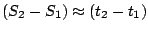 . In other words, if the infectee
reseeded twice, then the value of the seeds must differ by approximately
the same amount as the difference in milliseconds in the timestamps of
the two packets seen immediately after these reseedings at the
telescope. Extending this reasoning to . In other words, if the infectee
reseeded twice, then the value of the seeds must differ by approximately
the same amount as the difference in milliseconds in the timestamps of
the two packets seen immediately after these reseedings at the
telescope. Extending this reasoning to  reseeding events,
we get reseeding events,
we get  , ,  . This implies that the points . This implies that the points  should (approximately)
lie along a straight line with slope 1 (angle of should (approximately)
lie along a straight line with slope 1 (angle of  ) when plotting potential seed value against time. ) when plotting potential seed value against time.
We now describe a
geometric algorithm to detect such a set of points in a 2-dimensional
plane. The key observation is that when points lie close
to a straight line of a given slope, then looking from any one of these
points along that slope, the remaining points should appear clustered in
a very narrow band. More formally, if we project an angular beam of
width  from any one of these points, then the
remaining points should lie within the beam, for reasonably small values
of . On the other hand, other, randomly
scattered points on the plane will see a very small number of other
points in the beam projected from them. from any one of these points, then the
remaining points should lie within the beam, for reasonably small values
of . On the other hand, other, randomly
scattered points on the plane will see a very small number of other
points in the beam projected from them.
The algorithm
follows directly from this observation. It proceeds in iterations.
Within an iteration, we project a beam of width  along the line from each point in the plane. The point is
assigned a score equal to the number of other points that lie in its
beam. Actual seeds are likely to get a high score because they would all
lie roughly along a line. At the end of the iteration, all points with
a score smaller than some threshold (say along the line from each point in the plane. The point is
assigned a score equal to the number of other points that lie in its
beam. Actual seeds are likely to get a high score because they would all
lie roughly along a line. At the end of the iteration, all points with
a score smaller than some threshold (say  ) are
discarded. Repeating this process in subsequent iterations quickly
eliminates all but the seeds, which keep supporting
high scores for each other in all iterations. ) are
discarded. Repeating this process in subsequent iterations quickly
eliminates all but the seeds, which keep supporting
high scores for each other in all iterations.
Figure 11: Number of infectees
with a system uptime of the given number of days.
![\includegraphics[height=1.25in,width=3.0in]{plots/uptime784.eps}](img91.png) |
We find this
algorithm highly effective given enough reseeding events. Figure 11 presents the results of the computation of
system uptime of 784 machines in the infectee population. These
infectees were chosen from the set that contributed enough packets to
allow us to use our mechanism for estimating the seed. Since the
counter used by Witty to reseed its PRNG is only 32 bits wide, it will
wrap-around every milliseconds, which is approximately
49.7 days. The results could potentially be distorted due to this
effect (but see below).
There is a clear
domination of short-lived machines, with approximately 47% having
uptimes of less than five days. On the other hand, there are just five
machines that had an uptime of more than 40 days. The sharp drop-off
above 40 days leads us to conclude that the effects due to the
wrapping-around of the counter are negligible.
The highest number
of machines were booted on the same day as the spread of the worm. There
are prominent troughs during the weekends -- recall that the worm was
released on a Friday evening Pacific Time, so the nearest weekend had
passed 5 days previously -- and heightened activity during the working
days.
One
feature that stands out is the presence of two modes, one at 29 days
and the second at 36/37 days. On further investigation, we found that
the machines in the first mode all belonged to a set of 135 infectees
from the same /16 address block, and traceroutes revealed they were
situated at a single US military installation. Similarly, machines in
the second mode belonged to a group of 81 infectees from another /16
address block, belonging to an educational institution. However, while
machines in the second group appeared at the telescope one-by-one
throughout the infection period, 110 of the 135 machines in the first
group appeared at the telescope within 10 seconds of Witty's onset.
Since such a fast spread is not feasible by random scanning of the
address space, the authors of [18]
concluded that these machines were either part of a hit-list or were
already compromised and under the control of the attacker. Because we
can fit the actions of these infectees with running the full Witty
code, including PRNG reseeding patterns that match the process of
overwriting disk blocks, this provides evidence that these machines
were not specially controlled by the attacker (unlike the Patient
Zero machine), and thus we conclude that they likely constitute a
hit-list. Returning then to the fact that these machines were all
rebooted exactly 29 days before the onset of the worm, we speculate
that the reboot was due to a facility-wide system upgrade; perhaps the
installation of system software such as Microsoft updates (a critical
update had been released on Feb. 10, about 10 days before the
simultaneous system reboots), or perhaps the installation of the
vulnerable ISS products themselves. We might then speculate that the
attacker knew about the ISS installation at the site (thus
enabling them to construct a hit-list), which, along with the
attacker's rapid construction of the worm indicating they likely knew
about the vulnerability in advance [21], suggests that the
attacker was an ISS ``insider.''
Table 2: Disk counts of 100 infectees.
| Number of Disks |
1 |
2 |
3 |
4 |
5 |
6 |
7 |
| Number of Infectees |
52 |
32 |
12 |
2 |
2 |
0 |
0 |
|
Number of disks.
Once we can recover the seed used at the beginning of a sequence of
packets, we can use its value as an anchor to mark off the precise
subsequent actions of the worm. Recall from Fig. 2
that the worm generates exactly 20,000 packets in its inner loop, using
80,000 random numbers in the process. After exiting the inner loop, the
worm uses three bits from the next random number to decide which
physical disk it will attempt to open. Starting from the seed, this is
exactly the 80,001th number in the sequence generated by the PRNG. Thus,
knowledge of the seed tells us exactly which disk the worm attempts to
open. Furthermore, as discussed above we can tell whether this attempt
succeeded based on whether the worm reseeds after the attempt. We can
therefore estimate the number of disks on the infectee, based on which
of the attempts for drives in the range 0 to 7 lead to a successful
return from the open system call. Table 2
shows the number of disks for 100 infectees, calculated using this
approach. The majority of infectees had just one or two disks, while we
find a few with up to five disks. Since the installation of end-system
firewall software was a prerequisite for infection by Witty, the
infectee population is more likely to contain production servers with
multiple disks.
Exploration of
infection graph. Knowledge of the precise seeds allows us to
reconstruct the complete list of packets sent by each infectee.
Additionally, the large size of our telescope allows us to detect an
infectee within the first few seconds (few hundred packets) of its
infection. Therefore if an infectee is first seen at a time  , we can inspect the list of packets sent by all other
infectees active within a short preceding interval, say , we can inspect the list of packets sent by all other
infectees active within a short preceding interval, say  sec sec , to see which sent a packet
to the new infectee, and thus is the infectee's likely ``infector.'' to
select the most likely ``infector''. , to see which sent a packet
to the new infectee, and thus is the infectee's likely ``infector.'' to
select the most likely ``infector''.
The probability of
more than one infectee sending a worm packet to the same new infectee at
the time of its infection is quite low. With about 11,000 pkts/sec seen
at a telescope with 1/256 of the entire Internet address space, and
suffering 30% losses due to congestion (§ 5),
the aggregate scanning rate of the worm comes out to around  pkts/sec. With
more than pkts/sec. With
more than  addresses to scan, the probability that more than one infectee scans the
same address within the same 10 second interval is around 1%.
addresses to scan, the probability that more than one infectee scans the
same address within the same 10 second interval is around 1%.
Figure 12: Scans from infectees,
targeted to other victims.
![\includegraphics[scale=0.67]{plots/infect2.eps}](img97.png) |
Figure 13: Number of scans in 10
second buckets.
![\includegraphics[scale=0.67]{plots/diff.eps}](img98.png) |
Figure 12 shows scan packets from infected sources that
targeted other infectees seen at the telescope. The -coordinate
gives  , the packet's estimated sending
time, and the -coordinate gives the difference between , the packet's estimated sending
time, and the -coordinate gives the difference between  , the time when the target
infectee first appeared at the telescope, and . A small positive value of , the time when the target
infectee first appeared at the telescope, and . A small positive value of  raises strong suspicions that the given scan packet is responsible for
infecting the given target. Negative values mean the target was already
infected, while larger positive values imply the scan failed to infect
the target for some reason -- it was lost, (Recall that the effective
bandwidth of most infectees is much lower than the access bandwidth,
indicating heavy loss in their generated traffic.) or blocked due to the
random destination port it used, or simply the target was not connected
to the Internet at that time. (Note that the asymptotic curves at the
top and bottom correspond to truncation effects reflecting the upper and
lower bounds on infection times.)
raises strong suspicions that the given scan packet is responsible for
infecting the given target. Negative values mean the target was already
infected, while larger positive values imply the scan failed to infect
the target for some reason -- it was lost, (Recall that the effective
bandwidth of most infectees is much lower than the access bandwidth,
indicating heavy loss in their generated traffic.) or blocked due to the
random destination port it used, or simply the target was not connected
to the Internet at that time. (Note that the asymptotic curves at the
top and bottom correspond to truncation effects reflecting the upper and
lower bounds on infection times.)
The clusters at
extreme values of
in Figure 12 mask a very sharp additional
cluster, even using the log-scaling. This lies in the region  .
In Figure 13, we plot the number of scans in
10 second buckets against .
The very central sharp peak corresponds to the interval 0-to-10 seconds
-- a clear mark of the dispatch of a successful scan closely followed by
the appearance of the victim at the telescope. We plan to continue our
investigation of infector-infectee relationships, hoping to produce an
extensive ``lineage'' of infection chains for use in models of worm
propagation. .
In Figure 13, we plot the number of scans in
10 second buckets against .
The very central sharp peak corresponds to the interval 0-to-10 seconds
-- a clear mark of the dispatch of a successful scan closely followed by
the appearance of the victim at the telescope. We plan to continue our
investigation of infector-infectee relationships, hoping to produce an
extensive ``lineage'' of infection chains for use in models of worm
propagation.
7 Discussion
While we have
focused on the Witty worm in this paper, the key idea is much broader.
Our analysis demonstrates the potential richness of information embedded
in network telescope observations, ready to be revealed if we can frame
a precise model of the underlying processes generating the
observations. Here we discuss the breadth and limitations of our
analysis, and examine general insights beyond the specific instance of
the Witty worm.
Candidates for
similar analysis. The binary code of all Internet worms is available
by definition, making them candidates for disassembly and analysis.
Similarly, copies of many scanning and flooding tools have been captured
by white hat researchers, and traces observed at telescopes of probing
or attack traffic (or backscatter) from the operation of such tools
provide candidates for similar analysis. A preliminary assessment we
performed of ten well-known DoS attack tools revealed that six of them
use simple PRNGs with unsophisticated seeds, while the other four use
no random number generation at all. Even with limited knowledge of the
operation of such tools, we should in principle be able to analyze logs
of their attack traffic or backscatter with a similar intent of
reconstructing the sequence of events in the automation of the attack,
potentially leading to information about the attacking hosts, their
interaction with the network, and other forensic clues.
Diversity of
PRNGs. Our analysis was greatly facilitated by the use of a linear
congruential PRNG by Witty's author. Reverse-engineering the state of a
more complex PRNG could be much more difficult. In the extreme, a worm
using a cryptographically strong hash function with a well-chosen key as
its PRNG would greatly resist such reverse engineering. However, there
are several practical reasons that support the likelihood of many
attackers using simpler PRNGs.
Implementing good
PRNGs is a complicated task [8],
especially when constrained by limits on code size and the difficulty
of incorporating linkable libraries. Large-scale worms benefit greatly
from as self-contained a design as possible, with few dependencies on
platform support, to maximize the set of potential victims. Worms have
also proven difficult to fully debug -- virtually all large-scale worms
have exhibited significant bugs -- which likewise argues for keeping
components as simple as possible. Historically, worm authors have
struggled to implement even the LC PRNG correctly. The initial version
of Code Red failed to seed the PRNG with any entropy, leading to all
copies of the worm scanning exactly the same sequence of addresses [2]. Slammer's PRNG
implementation had three serious errors, one where the author used a
value of the parameter in the LC equation (Eqn. 1) that was larger than the correct value by 1 due to
an incorrect 2's complement conversion, another where this value was
subtracted from instead of added to the term  in Eqn 1, and finally the (mis)use of an OR instruction
rather than XOR to clear a key register [11]. In addition, sources
of local entropy at hosts are often limited to a few system variables,
complicating the task of seeding the PRNG in a fashion strong enough to
resist analysis. Thus it is conceivable that worm authors will have
difficulty implementing bug-free, compact versions of sophisticated
PRNGs. in Eqn 1, and finally the (mis)use of an OR instruction
rather than XOR to clear a key register [11]. In addition, sources
of local entropy at hosts are often limited to a few system variables,
complicating the task of seeding the PRNG in a fashion strong enough to
resist analysis. Thus it is conceivable that worm authors will have
difficulty implementing bug-free, compact versions of sophisticated
PRNGs.
In addition,
today's worm authors have little incentive to implement a complex PRNG.
As long as their goals are confined to effectively scanning the IP
address space and maximizing the worm's infection rate, simple PRNGs
suffice. Hiding one's tracks while releasing a worm can already be
accomplished by using a chain of compromised victims as stepping stones.
Indeed, the fact that Witty's author left Patient Zero running
with a separate program for spreading the worm was purely a mistake on
his/her part. As discussed earlier, the code it ran scanned a very
small subset of the IP address space, and did not manage to produce
even one infection during scanning.
Thus, there are
significant factors that may lead to the continued use by worms of
simple PRNGs such as LC, which, along with the availability of
disassembled code, will facilitate the development of structural models
of worm behavior to use in conjunction with telescope observations for
detailed reconstructions.
General
observations from this work. Our study has leveraged the special
conditions produced by a worm's release to measure numerous features of
its victim population and the network over which it spread. While
specific estimation tricks developed in this paper might not apply to
other telescope observations in a ``cookbook'' manner, the insight that
telescope observations carry rich information that can be heavily mined
armed with a sufficiently detailed model of the underlying source
processes is of major significance for the future study of such data.
Understanding the
structure of the scanning techniques used by worms (and empirical data
on hitherto unmeasured quantities such as distribution of access
bandwidth) can be crucial for developing correct models of their spread
-- a case made for example by our observation of the doubly-scanned and
never-scanned portions of the address space, and their multi-factored
impact on the worm's growth.
Finally, we would
emphasize that the extraction of the features we have assessed was a
labor-intensive process. Indeed, for many of them we did not initially
apprehend even the possibility of analyzing them. This highlights not
only the difficulty of such a forensic undertaking, but also its
serendipitous nature. The latter holds promise that observations of
other Internet-scale events in the future, even those of significantly
different details or nature, will likely remain open to the possibility
of such analysis.
8 Conclusions
A worm's
propagation is a rare but spectacular event in today's networks. Apart
from the obvious disruptions and damage, worms also stress the network
in unique ways and at scales unmatched by any controlled measurement
experiments. One could say that a worm's release illuminates, for a few
moments, dark corners of the network just as supernovae illuminate dark
and distant corners of the universe, providing rich observations to
telescopes that gather a mere sliver of the enormous radiant flux. But
within the overwhelming mass of observed data lies a very structured
process that can be deciphered and understood -- if studied with the
correct model.
We have shown how a
fine-grained understanding of the exact control flow of a particular
worm -- especially its seeding and use of a pseudo-random number
generator -- when coupled with network telescope data enables a detailed
reconstruction of nearly the entire chain of events that followed the
worm's release. In the process we have unearthed measurements of
quantities such as access bandwidth and system up-time that are
otherwise unobservable to the ``naked eye'' of researchers studying
systems from afar. These measurements have applicability to a number of
modeling and simulation studies, both in particular to worm propagation
analysis, and more generally as a source of rarely-available empirical
data. Finally, we have demonstrated the forensic power that such
analysis can provide, marshalling strong evidence that the Witty worm
specifically targeted a US military base and was launched via an IP
address corresponding to a European ISP. We investigated an alternate
explanation that instead these machines were passively monitoring large
address regions and hence were infected much more quickly, but can
discount this possibility because a ``lineage'' analysis reveals that a
significant number of the machines did not receive any infection
packets on even their entire local /16 prior to their own scanning
activity arriving at the telescope.
Acknowledgments
This
work was supported by the National Science Foundation under the
following grants: Collaborative Cybertrust NSF-0433702, ITR/ANI-0205519,
NRT-0335290, and ANI-0238315, for which we are grateful. We thank
Colleen Shannon and David Moore at CAIDA, and Paul Barford and Vinod
Yegneswaran at the University of Wisconsin for providing access to the
telescope traces and answering numerous questions about them, and our
CCIED colleagues and Ellen Zegura for valuable feedback.
Support
for the Witty Worm Dataset and the UCSD Network Telescope are provided
by Cisco Systems, Limelight Networks, the US Dept. Homeland Security,
the National Science Foundation, and CAIDA, DARPA, Digital Envoy, and
CAIDA Members.
-
- 1
- Michael Bailey, Evan Cooke, Farnam Jahanian, Jose Nazario, and
David Watson.
The Internet motion sensor: A distributed blackhole monitoring system.
In Proc. NDSS, 2005.
- 2
- CAIDA.
CAIDA Analysis of Code-Red,
https://www.caida.org/analysis/security/code-red/
- 3
- CERT.
CERT Advisory CA-1999-04 Melissa Macro Virus,
https://www.cert.org/advisories/CA-1999-04.html
- 4
- Evan Cooke, Michael Bailey, Z. Morley Mao, David Watson, Farnam
Jahanian, and Danny McPherson.
Toward understanding distributed blackhole placement.
In Proc. ACM CCS Workshop on Rapid Malcode (WORM), October
2004.
- 5
- Domas Mituzas.
FreeBSD Scalper Worm, https://www.dammit.lt/apache-worm/
- 6
- eEye Digital Security.
.ida ``Code Red'' Worm,
https://www.eeye.com/html/Research/Advisories/AL20010717.html.
- 7
- Mark Eichin and Jon Rochlis.
With microscope and tweezers: An analysis of the Internet virus of
november 1988.
In Proc. IEEE Symposium on Research in Security and Privacy,
1989.
- 8
- Donald E. Knuth.
The Art of Computer Programming, Second Edition, volume 2,
Seminumerical Algorithms.
Addison-Wesley, 1981.
- 9
- K. Kortchinsky.
Black Ice worm disassembly.
https://www.caida.org/analysis/security/witty/BlackIceWorm.html.
- 10
- D. Moore, C. Shannon, G. Voelker, and S. Savage.
Network telescopes: Technical report.
Technical report, Cooperative Association for Internet Data Analysis
(CAIDA), July 2004.
- 11
- David Moore, Vern Paxson, Stefan Savage, Colleen Shannon, Stuart
Staniford, and Nicholas Weaver.
Inside the Slammer Worm.
IEEE Security & Privacy, pages 33-39, July/August
2003.
- 12
- David Moore, Vern Paxson, Stefan Savage, Colleen Shannon, Stuart
Staniford, and Nicholas Weaver.
The Spread of the Sapphire/Slammer Worm, 2003.
- 13
- David Moore, Colleen Shannon, and k claffy.
Code-Red: a Case Study on the Spread and Victims of an Internet Worm.
In Proceedings of the Second Internet Measurement Workshop,
pages 273-284, November 2002.
- 14
- David Moore, Geoffrey M. Voelker, and Stefan Savage.
Inferring Internet Denial-of-Service Activity.
In Proceedings of the 10th USENIX Security Symposium, pages
9-22. USENIX, August 2001.
- 15
- Ruoming Pang, Vinod Yegneswaran, Paul Barford, Vern Paxson, and
Larry Peterson.
Characteristics of Internet background radiation.
In Proc. ACM Internet Measurement Conference, October 2004.
- 16
- F secure Inc.
Global slapper worm information center, https://www.f-secure.com/slapper/
- 17
- C. Shannon and D. Moore.
The caida dataset on the witty worm, March 19-24 2004.
https://www.caida.org/passive/witty/.
- 18
- C. Shannon and D. Moore.
The spread of the Witty worm.
IEEE Security and Privacy, 2(4):46-50, August 2004.
- 19
- Eugene Spafford.
The Internet worm program: An analysis. purdue technical report
csd-tr-823, 1988.
- 20
- Stuart Staniford and Vern Paxson and Nicholas Weaver.
How to 0wn the Internet in Your Spare Time.
In Proceedings of the 11th USENIX Security Symposium. USENIX,
August 2002.
- 21
- Nicholas Weaver and Dan Ellis.
Reflections on Witty: Analyzing the attacker.
;login:, pages 34-37, June 2004.
- 22
- V. Yegneswaran, P. Barford, and D. Plonka.
On the design and utility of Internet sinks for network abuse
monitoring.
In Proc. of Symposium on Recent Advances in Intrusion Detection,
September 2004.
- 23
- Cliff Changchun Zou, Weibo Gong, and Don Towsley.
Code Red Worm Propagation Modeling and Analysis.
In Proceedings of the ACM CCS 2002 conference, November 2002.
|


![\includegraphics[scale=0.6]{plots/growthrate.eps}](img43.png)
![\includegraphics[scale=0.7]{plots/fullhr.eps}](img55.png)
![\includegraphics[scale=0.67]{plots/compare.eps}](img59.png)
![\includegraphics[scale=0.7]{plots/caidaextra2.eps}](img61.png)
![\includegraphics[scale=0.67]{plots/compcaidaextra.eps}](img62.png)
![\includegraphics[scale=0.67]{plots/pktrate2.eps}](img66.png)
![\includegraphics[scale=0.67]{plots/compextraboth.eps}](img68.png)