FAST '05 Paper [FAST '05 Technical Program]

MicroHash: An Efficient Index Structure for
Flash-Based Sensor Devices

Demetrios Zeinalipour-Yazti, Song Lin, Vana Kalogeraki, Dimitrios Gunopulos, Walid A. Najjar

Dept. of Computer Science Dept. of Computer Science & Engineering

University of Cyprus University of California, Riverside

dzeina@cs.ucy.ac.cy {slin,vana,dg,najjar}@cs.ucr.edu

Abstract

In this paper we propose the MicroHash index, which is an efficient external memory structure for Wireless Sensor Devices (WSDs). The most prevalent storage medium for WSDs is flash memory. Our index structure exploits the asymmetric read/write and wear characteristics of flash memory in order to offer high performance indexing and searching capabilities in the presence of a low energy budget which is typical for the devices under discussion. A key idea behind MicroHash is to eliminate expensive random access deletions. We have implemented MicroHash in nesC, the programming language of the TinyOS [7] operating system. Our trace-driven experimentation with several real datasets reveals that our index structure offers excellent search performance at a small cost of constructing and maintaining the index.

1 Introduction

The improvements in hardware design along with the wide availability of economically viable embedded sensor systems enable researchers nowadays to sense environmental conditions at extremely high resolutions. Traditional approaches to monitor the physical world include passive sensing devices which transmit their readings to more powerful processing units for storage and analysis. Wireless Sensor Devices (WSDs) on the other hand, are tiny computers on a chip that is often as small as a coin or a credit card. These devices feature a low frequency processor ( $\approx$ 4-58MHz) which significantly reduces power consumption, a small on-chip flash memory ( $\approx$ 32KB-512KB) which can be used as a temporary local storage medium, a wireless radio for communication, on-chip sensors, and an energy source such as a set of AA batteries or solar panels [13]. This multitude of features constitute WSDs powerful devices which can be used for in-network processing, filtering and aggregation [11,12,16]. Large-scale deployments of sensor network devices have already emerged in environmental and habitant monitoring [13,15], seismic and structural monitoring [24], factory and process automation and a large array of other applications [11,12,16].

In long-term deployments, it is often cheaper to keep a large window of measurements in-situ (at the generating site) and transmit the respective information to the user only when requested (this is demonstrated in Section 2.4). For example, biologists analyzing a forest are usually interested in the long-term behavior of the environment. Therefore the sensors are not required to transmit their readings to a sink (querying node) at all times. Instead, the sensors can work unattended and store their reading locally until certain preconditions are met, or when the sensors receive a query over the radio that requests the respective data. Such in-network storage conserves energy from unnecessary radio transmissions, which can be used to increase the sampling frequency of the data and hence the fidelity of the measurements in reproducing the actual physical phenomena and prolong the lifetime of the network.

Currently, the deployment of the sensor technology is severely hampered by the lack of efficient infrastructure to store locally large amounts of sensor data measurements. The problem is that the local RAM memory of the sensor nodes is both volatile and very limited ( $\approx$ 2KB-64KB). In addition, the non-volatile on-chip flash memory featured by most sensors is also very limited ( $\approx$ 32KB-512KB). However the limited local storage of sensor devices is expected to change soon. Several sensor devices, such as the RISE [1] hardware platform, include off-chip flash memory which supplements each sensor with several megabytes of storage. Flash memory has a number of distinct characteristics compared to other storage media: First, each page (typically 128B-512B) can only be written a limited number of times ( $\approx$ 10,000-100,000). Second, pages can only be written after they have been deleted in their entirety. However, a page deletion always triggers the deletion of its respective block ( $\approx$ 8KB-64KB per block). Due to these fundamental constraints, efficient storage management becomes a challenging task.

The problem that we investigate in this paper is how to efficiently organize the data locally on flash memory. Our desiderata are:

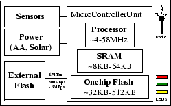
To provide efficient access to the data stored on flash by time or value, for equality queries generated by the user.
To increase the longevity of the flash memory by spreading page writes out uniformly so that the available storage capacity does not diminish at particular regions of the flash media.

We propose the MicroHash index, which serves as a primitive structure for efficiently indexing temporal data and for executing a wide spectrum of queries. Note that the data generated by sensor nodes has two unique characteristics: i) Records are generated at a given point in time (i.e. these are temporal records), and ii) The recorded readings are numeric values in a limited range. For example a temperature sensor might only record values between -40F to 250F with one decimal point precision. Traditional indexing methods used in relational database systems are not suitable as these do not take into account the asymmetric read/write behavior of flash media. Our indexing techniques have been designed for sensor nodes that feature large flash memories, such as the RISE [1] sensor, which provide them with several MBs of storage. MicroHash has been implemented in nesC [6] and uses the TinyOS [7] operating system.

In this paper we make the following contributions:

We propose the design and implementation of MicroHash, a novel index structure for supporting equality queries in sensor nodes with limited processing capabilities and a low energy budget.
We present efficient algorithms for inserting, deleting and searching data records stored on flash.
We describe the prototype implementation of MicroHash in nesC [6], and demonstrate the efficiency of our approach with an extensive experimental study using atmospheric readings from the University of Washington [21] and the Great Duck Island study [15].

2 The Memory Hierarchy

In this section we briefly overview the architecture of a sensor node, with a special focus on its memory hierarchy. We also study the distinct characteristics of flash memory and address the challenges with regards to energy consumption and access time.

2.1 System Architecture

The architecture of a sensor node (see Figure 1), consists of a microcontroller unit (MCU) which is interconnected to the radio, the sensors, a power source and the LEDs. The MCU includes a processor, a static RAM (SRAM) module and an on-chip flash memory. The processor runs at low frequencies ( $\approx$ 4-58MHz) which reduces power consumption. The SRAM is mainly used for code execution while in the latest generation of sensors, such as Yale's 58MHz XYZ node [10] and the Intel's 12MHz iMote (https://www.intel.com), it can also be used for in-memory (or SRAM) buffering. The choice of the right energy source is application specific. Most sensors either deploy a set of AA batteries or solar panels [13]. Therefore a sensor node might have a very long lifetime.

**Figure:** The Architecture of a typical Wireless Sensor.
$\begin{figure}\begin{center} \epsfig{figure=figs/sensor.eps,width=2.2in}\end{center}\end{figure}$

The on-chip flash provides a small non-volatile storage area (32KB-512KB) for storing the executable code or for accumulating values for a small window of time [11]. A larger external storage can also be supplemented to a sensor using the Serial Peripheral Interface (SPI) which is typically found on these devices. For example in the RISE platform, nodes feature a larger off-chip flash memory which provides the sensor with several MBs of storage. The external flash memory is connected to the MCU through a Serial Peripheral Interface (SPI), that operates at a fraction of the CPU frequency (e.g. ${\frac{{cpufreq}}{{8}}}$ ). Therefore a faster processor would increase the maximum throughput of the SPI interface.

Although it is currently not clear whether Moore's Law will apply to the size and price of the sensor units or their hardware characteristics, we believe that future sensor nodes will feature more SRAM and flash storage, as more complex in-network processing applications, increase the memory and potentially the CPU demand.

2.2 Overview of Flash Memory

Flash Memory is the most prevalent storage media used in current sensor systems because of its many advantages including: i) non-volatile storage, ii) simple cell architecture, which allows easy and economical production, iii) shock-resistance, iv) fast read access and power efficiency. These characteristics establish flash memory as an ideal storage media for mobile and wireless devices [3].

There are two different types of flash memory, NOR flash and NAND flash, which are named according to the logic gate of their respective storage cell. NAND flash is the newer generation of flash memory which is characterized by faster erase time, higher durability and higher density. NOR is an older type of flash which is mainly used for code storage (e.g. for the BIOS). Its main advantage is that it supports writes at a byte granularity as opposed to page granularity used in NAND flash. NOR flash has also faster access time (i.e. $\approx$ 200ns) than NAND (50-80 $\mu$ s) but lacks in all other characteristics such as density and power efficiency.

For the rest of the paper we will focus on the characteristics of NAND memory as this is the type of memory used for the on-chip and off-chip flash of most sensors including the RISE platform. According to Micron (https://www.micron.com/), NAND memory is the fastest growing memory market in 2005 ($8.7 billion). NAND flash features a number of distinct constraints which can be summarized as following:

Read-Constraint: Reading data stored on flash memory can be performed at granularities ranging from a single byte to a whole block (typically 8KB-64KB).
Delete-Constraint: Deleting data stored on flash memory can only be performed at a block granularity (i.e. 8KB-64KB).
Write-Constraint: Writing data can only be performed at a page granularity (typically 256B-512B), after the respective page (and its respective 8KB-64KB block) has been deleted.
Wear-Constraint: Each page can only be written a limited number of times (typically 10,000-100,000).

The design of our MicroHash index structure in Section 5, considers the above constraints.

Table: Performance Parameters for NAND Flash using a 3.3V voltage, 512B Page size and 16KB Block size

NAND Flash installed on a Sensor Node
	Page Read	Page Write	Block Erase
	1.17mA	37mA	57mA
Time	6.25ms	6.25ms	2.26ms
Data Rate	82KBps	82KBps	7MBps
Energy	24 $\mu$ J	763 $\mu$ J	425 $\mu$ J
	Page Erase-Write	Flash Idle	Flash Sleep
	43mA	0.068mA	0.031mA
Time	6.75ms	N/A	N/A
Data Rate	76KBps	N/A	N/A
Energy	957 $\mu$ J	220 $\mu$ J/sec	100 $\mu$ J/sec

2.3 Access Time of NAND Flash

Table 1, presents the average measurements that we obtained from a series of micro-benchmarks using the RISE platform along with a HP E3630A constant 3.3V power supply and a Fluke 112 RMS Multimeter. The first observation is that reading is three orders of magnitude less power demanding than writing. On the other hand, block erases are also quite expensive but can be performed much faster than the former two operations. Note that read and write operations involve the transfer of data between the MCU and the SPI bus, which becomes the bottleneck in the time to complete the operation. Specifically, reading and writing on flash media without the utilization of the SPI bus can be achieved in $\approx$ 50 $\mu$ and $\approx$ 200 $\mu$ s respectively [22]. Finally, our results are comparable to measurements reported for the MICA2 mote in [2] and the XYZ sensor in [10].

Although these are hardware details, the application logic needs to be aware of these characteristics in order to minimize energy consumption and maximize performance. For example, the deletion of a 512B page will trigger the deletion of a 16KB block on the flash memory. Additionally the MCU has to re-write the rest unaffected 15.5KB. One of the objectives of our index design is to provide an abstraction which hides these hardware specific details from the application.

2.4 Energy Consumption of NAND Flash

Another question is whether it is cheaper to write to flash memory rather than transmitting over the RF radio. We used the RISE mote to measure the cost of transmitting the data over a 9.6Kbps radio (at 60mA), and found that transmitting 512B (one page) takes on average 416ms or 82,368 $\mu$ J. Comparing this with the 763 $\mu$ J required for writing the same amount of data to local flash, along with the fact that transmission of one byte is roughly equivalent to executing 1120 CPU instructions, makes local storage and processing highly desirable.

A final question we investigated is how many bytes we can store on local flash before a sensor runs out of energy. Note that this applies only to the case where the sensor runs on batteries. Double batteries (AA) used in many current designs operate at a 3V voltage and supply a current of 2500 mAh (milliAmp-hours). Assuming similarly to [15], that only 2200mAh is available and that all current is used for data logging, we can calculate that AA batteries offer 23, 760J (2200mAh * 60 * 60 * 3). 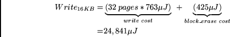With a 16KB block size and a 512B page size, we would have one block delete every 32 page writes (16KB/512B). Writing a page, according to our measurements, requires 763 $\mu$ J while the cost of performing a block erase is 425 $\mu$ J. Therefore writing 16KB requires:

Using the result from the above equation, we can derive that by utilizing the 23, 760J offered by the batteries, we can write $\approx$ 15GB before running out of batteries ((23,760J * 16KB) / 24,841 $\mu$ J). An interesting point is that even in the absence of a wear-leveling mechanism we would be able to accommodate the 15GB without exhausting the flash media. However this would not be true if we used solar panels [13], which provide a virtually unlimited power source for each sensor device. Another reason why we want to extend the lifetime of the flash media is that the batteries of a sensor node could be replaced in cases where the devices remain accessible.

3 Problem Definition

In this section we provide a formal definition of the indexing problem that the MicroHash index addresses. We also describe the structure of the MicroHash index and explain how it copes with the distinct characteristics of flash memory.

Let S denote some sensor that acquires readings from its environment every $\epsilon$ seconds (i.e. t = 0, $\epsilon$ , 2 $\epsilon$ ,...). At each time instance t, the sensor S obtains a temporal data record drec = { $\underline{{t}}$ , v₁, v₂,..., v_x}, where t denotes the timestamp (key) on which the tuple was recorded, while v_i ( 1 $\leq$ i $\leq$ x) represents the value of some reading (such as humidity, temperature, light and others).

Also let P = {p₁, p₂,..., p_n} denote a flash media with n available pages. A page can store a finite number of bytes (denoted as p^size_i), which limits the capacity of P to $\sum_{{i=0}}^{{n}}$ p^size_i. Pages are logically organized in b blocks {block₁, block₂,..., block_b}, each block containing n/b consecutive pages. We assume that pages are read on a page-at-a-time basis and that each page p_i can only be deleted if its respective block (denoted as p^block_i) is deleted as well (write/delete-constraint). Finally due to the wear-constraint, each page can only be written a limited number of times (denoted as p^wc_i).

The MicroHash index supports efficient value-based equality queries and efficient time-based equality and range queries. These queries are defined as follows:

Definition 1 Value-Based Equality Queries: A One dimensional query Q(v_i, a) in which the field values of attribute v_i are equivalent to value a.

For example the query q= (temperature, 95F) can be used to find time instances (ts) and other recorded readings when the temperature was 95F.

Definition 2 Time-Based Range and Equality Queries: A range query is a one dimensional query Q(t, a, b) in which the time attribute t, is between the lower and upper bound a and b respectively. The equality query is a special case of the range query Q(t, a, b) in which a = b.

For example the query q= (ts, 100, 110) can be used to find the tuples recorded in the 10 second interval.

Evaluating the above queries efficiently requires that the system maintains an index structure along with the generated data. Specifically, while a node senses data from its environment (i.e. data records), it also creates index entries that point to the respective data stored on the flash media. When a node needs to evaluate some query, it uses the index records to quickly locate the desired data. Since the number of index records might be potentially very large, these are stored on the external flash as well. Although maintaining index structures is a well studied problem in the database community [4,9,19], the low energy budget of sensor nodes along with the unique read, write, delete and wear constraints of flash memory introduce many new challenges. In order to maximize efficiency our design objectives are as follows:

Wear-Leveling: Spread page writes out uniformly across the storage media P in order to avoid wearing out specific pages.
Block-Erase: Minimize the number of random-access deletions as the deletion of individual pages triggers the deletion of the whole respective block.
Fast-Initialization: Minimize the size of in-memory (SRAM) structures that will be required in order to use the index.

4 MicroHash Data Structures

In this section we describe the data structures created in the fast but volatile SRAM to provide an efficient way to access data stored on the persistent but slower flash memory. First we describe the underlying organization of data on the flash media and then describe the involved in-memory data structures.

4.1 Flash Organization

MicroHash uses a Heap Organization, in which records are stored on the flash media in a circular array fashion. This allows data records to be naturally sorted based on their timestamp and therefore our organization is Sorted by Timestamp. This organization requires the least overhead in SRAM (i.e. only one data write-out page). Additionally, as we will show in Section 5.4, this organization addresses directly the delete, write and wear constraint. When the flash media is full we simply delete the next block following idx. Although other organizations in relational database systems, such as Sorted or Hashed on some attribute could also be used, they would have a prohibitive cost as the sensor would need to continuously update written pages (i.e. perform an expensive random page write). On the other hand, our Heap Flash Organization always yields completely full data pages as data records are consecutively packed on the flash media.

4.2 In-Memory (SRAM) Data Structures

The flash media is segmented into n pages, each with a size of 512B. Each page consists of a 8B header and a 504B payload.

Specifically the header includes the following fields (also illustrated in Figure 2):
i) A 3-bit Page Type (TYP) identifier, used to for the different types of pages (data, index, directory and root). ii) A 16-bit Cyclic Redundancy Checking (CRC) polynomial on the payload, which can be used for integrity checking. iii) A 7-bit Number of Records (SIZ), which identifies how many records are stored inside a page. We use fixed size records because records generated by a sensor always have the same size. iv) A 23-bit Previous Page Address (PPA), stores the address of some other page on the flash media giving in that way the capability to create linked lists on the flash. v) A 15-bit Page Write Counter (PWC), which keeps the number of times a page has been written to flash.

While the header is identical for any type of page, the payload can store four different types of information:
i) Root Page: contains information related to the state of the flash media. For example it contains the position of the last write (idx), the current cycle (cycle) and meta-information about the various indexes stored on the flash media. ii) Directory Page: contains a number of directory records (buckets) each of which contains the address of the last known index page mapped to this bucket. In order to form larger directories several directory pages might be chained using the 23-bit PPA address in the header. iii) Index Page: contains a fixed number of index records and the 8 byte timestamp of the last known data record. The latter field, denoted as anchor is exploited by timestamp searches which can make an informed decision on which page to follow next. Additionally, we evaluate two alternative index record layouts. The first, denoted as offset layout, maintains for each data record a respective pageid and offset, while the second layout, denoted as nooffset, maintains only the pageid of the respective data record. iv) Data Page: contains a fixed number of data records. For example when the record size is 16B then each page can contain 31 consecutively packed records.

Figure 2: Main data structures used in our nesC implementation of the MicroHash Index.

	typedef struct Page {
		uint8_t 	typ:3;
		uint16_t 	crc:16;
		uint16_t	pwc:15;
		uint8_t     siz:7;
		uint32_t    ppa:23;
		union {
		  RootP	rootP;
		  DirP	dirP;
		  IdxP  idxP;
		  DataP dataP;
		};
	} __attribute__((packed));

	typedef struct IdxP {
		// optional anchor
		uint64_t lastTS;
		IdxRec records[IREC];
	} __attribute__((packed));

	typedef struct DataP {
		DataRec records[DREC];
	} __attribute__((packed));

	typedef struct DataRec {
		timestamp_t	ts;
		data_t  	val1;
	} __attribute__((packed));

	typedef struct IdxRec {
		fladdress_t	datap;
		// optional offset
		floffset_t	offset;
	} __attribute__((packed));

5 Indexing in MicroHash

The MicroHash index is an efficient external-memory structure designed to support equality queries in sensor nodes that have limited main memory and processing capabilities. A MicroHash index structure consists of two substructures: i) A Directory and ii) a set of Index Pages. The Directory consists of a set of buckets. Each bucket maintains the address of the newest (chronologically) index page that maps to that bucket. The Index Pages contain the addresses of the data records that map to the respective bucket. Note that there might be an arbitrarily large number of data and the index pages. Therefore these pages are stored on the flash media and fetched into main memory only when requested.

The MicroHash index is built while data is being acquired from the environment and stored on the flash media. In order to better describe our algorithm we divide its operation in four conceptual phases: a) The Initialization Phase in which the root page and certain parts of the directory are loaded into SRAM, b) The Growing Phase in which data and index pages are sequentially inserted and organized on the flash media, c) The Repartition Phase in which the index directory is re-organized such that only the directory buckets with the highest hit ratio remain in memory, and the d) The Deletion Phase which is triggered for garbage collection purposes.

5.1 The Initialization Phase

In the first phase the MicroHash index locates the root page on flash media. In our current design, the root page is written on a specific page on flash (page0). If page0 is worn out, we recursively use the next available page. Therefore a few blocks are pre-allocated at the beginning of the flash media for the storage of root pages. The root page indicates what type of indexes are available on the system and the addresses of their respective directories. Given that an application requires the utilization of an index I, the system pre-loads part of I's directory into SRAM (detailed discussion follows in Section 5.3). The root and directory pages then remain in SRAM, for efficiency, and are periodically written out to flash.

5.2 The Growing Phase

Let us assume that a sensor generates a temporal record drec = {t, v₁, v₂,..., v_x} every $\epsilon$ seconds, where t is the timestamp on which the record was generated and v_i ( 1 $\leq$ i $\leq$ x) some distinct reading (e.g. humidity, temperature, etc). Instead of writing drec directly to flash, we use an in-memory (SRAM) buffer page p^write. When p^write gets full it is flushed to the address idx, where idx denotes the address after the last page write. Note that idx starts out as zero and this counter is incremented by one every time a page is written out. When idx becomes equal to the size of the flash media n, it is reset to zero. In order to provide a mechanism for finding the relative chronological order of pages written on the flash media, we also maintain the counter cycle, which is incremented by one every time idx is reset to zero. The combination of the < cycle, pageid> provides this mechanism.

Next we describe how index records are generated and stored on the flash media. The index records in our structure are generated whenever the p^write gets full. At this point we can safely determine the physical address of the records in p^write (i.e. idx). We create one index record ir = [idx, offset] for each data record in p^write ( $\forall$ drec $\in$ p^write). For example assume that we insert the following 12 byte [timestamp, value] records into an empty MicroHash index: {[1000,50], [1001,52], [1002,52]}. This will trigger the creation of the following index records: { [0,0],[0,12],[0,24] }. Since p^write is written to address idx the index records always reference data records that have a smaller <cycle,pageid> identifier.

The MicroHash Directory provides the start address of the index pages. It is constructed by providing the following three parameters: a) A lower bound (lb) on the indexed attribute, b) an upper bound (ub) on the indexed attribute and the number of available buckets c (note that we can only fit a certain number of directory buckets in memory). For example assume that we index temperature readings which are only collected in the following known and discrete range [- 40..250], then we set lb = - 40F, ub = 250F and c = 100. Initially each bucket represents exactly ${\frac{{\vert lb..ub\vert}}{{c}}}$ consecutive values although this equal splitting (which we call equiwidth splitting) is refined in the repartition phase based on the data values collected at run-time.

5.3 The Repartition Phase

A drawback of the initial equiwidth bucket splitting approach is that some buckets may rarely be used while others may create long lists of index records. To overcome this problem, we use the following splitting policy: Whenever a directory bucket A links to more than $\tau$ records (user parameter), we evict to flash the bucket B, which was not used for the longest period of time. Note that this mechanism can be implemented using only two counters per bucket (one for the timestamp and one for the number of records). In addition to the eviction of page B, we also create a new bucket A1. Our objective is to provide a finer granularity to the entries in A as this bucket is the most congested one. Note that the values in A are not reassigned between A and A1 as it would happen in dynamic hashing techniques, such as extendible hashing [4] or linear hashing [9]. The reason is that the index pages are on the flash media and updating these pages would result in a potentially very large number of random updates (which would be extremely expensive). Our equidepth, rather than equiwidth, bucket splitting approach keeps in memory finer intervals for index records used more frequently.

Figure 3: The Repartition Phase.

$\epsfbox{figs/repartition.eps}$

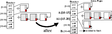
Figure 3 shows that each bucket is associated with a counter s, that indicates the timestamp of the last time the buffer was used, and a counter c that indicates the number of index records added since the last split. In the example, the c = 3 value in bucket 2 (A:[10-20]) exceeds the $\tau$ = 2 threshold and therefore the index forces bucket 4 (B:[30-40]) to the flash media while bucket two is split into A:[10-15] and A1:[15-20]. Note that the A list now contains values in [10-20] while the A1 list contains only values in the range [15-20].

5.4 The Deletion Phase

In this phase the index performs a garbage collection operation of the flash media in order to make space for new data. The phase is triggered after all n pages have been written to the flash media. This operation blindly deletes the next n/b pages (the whole next block starting at idx). It is then triggered again whenever n/b pages have been written, where b is the number of blocks on the flash media. That leaves the index with n/b clean pages that can be used for future writes. Note that this might leave pointers from index pages referencing data that is already deleted. This problem is handled by our search algorithm described in the next section.

The distinct characteristic of our garbage collection operation is that it satisfies directly the delete-constraint, because pages are deleted in blocks (which is cheaper than deleting a page-at-a-time). This makes it different from similar operations of flash file systems [2,17] that perform page-at-a-time deletions. Additionally, this mode provides the capability to "blindly" delete the next block without the need to read or relocate any of the deleted data. The correctness of this operation is established by the fact that the index records always reference data records that have a smaller <cycle,pageid> identifier. Therefore when an index page is deleted then we are sure that all associated data pages are already deleted.

6 Searching in MicroHash

In this section we show how records can efficiently be located by their value or timestamp.

6.1 Searching by Value

The first problem we consider is how to perform value-based equality queries. Finding records by their value involves: a) locating the appropriate directory bucket, from which the system can extract the address of the last index page, b) reading the respective index pages on a page-by-page basis and c) reading the data records referred by the index pages on a page-by-page basis. Since SRAM is extremely limited on a sensor node we adopt a record-at-a-time query return mechanism, in which records are reported to the caller on record-by-record basis. This mode of operation requires three available pages in SRAM, one for the directory (dirP) and two for the reading (idxP,dataP), which only occupies 1.5KB. If more SRAM was available, the results could have been returned at other granularities as well. The complete search procedure is summarized in Algorithm 1.

$\begin{algorithm} % latex2html id marker 281 [h] \begin{small} \caption{Equality... ...ignal $finished$; \par\EndProcedure \end{algorithmic}\end{small}\end{algorithm}$
Note that the loadPage procedure in line 4 and 6 returns NULL if the fetched page is not in valid chronological order (with respect to its preceding page) or, if the data records, in data pages, are not within the specified bucket range. This is consequence of the way the garbage collector operates, as it does not update the index records during deletions for performance reasons. However, these simple checks applied by loadPage ensure that we can safely terminate the search at this point. Finally, since the MicroHash index returns records on a record-at-a-time basis, we use a final signal finished which notifies the application that the search procedure has been completed.

6.2 Searching by Timestamp

In this section we investigate time-based equality and range queries. First, note that if index pages were stored in a separate physical location, and thus not interleaved with data pages, the sorted (by timestamp) file organization would allow us to access any data record in O(1) time. However, this would also violate our wear leveling mechanism as we wouldn't be able to spread out the page writes uniformly among data and index pages. Another approach would be to deploy an in-memory address translation table, such as the one used in [22] and [23], which would hide the details of wear-leveling mechanism. However, such a structure might be too big given the memory constraints of a sensor node and would also delay the sensor boot time.

Efficient search can be supported by a number of different techniques. One popular technique is to perform a binary search over all pages stored on the flash media. This would allow us to search in O(logn) time, where n is the size of the media. However, for large values of n such a strategy is still expensive. For example with a 512MB flash media and a page size of 512B we would need approximately 20 page reads before we find the expected record.

In our approach we investigate two binary search variants named: LBSearch and ScaleSearch. LBSearch starts out by setting a pessimistic lower bound on which page to examine next, and then recursively refines the lower bound until the requested page is found. ScaleSearch on the other hand exploits knowledge about the underlying distribution of data and index pages in order to offer a more aggressive search method that usually executes faster. ScaleSearch is superior to LBSearch when data and index pages are roughly uniformly distributed on the flash media but its performance deteriorates for skewed distributions.

For the remainder of this section we assume that a sensor S maintains locally some indexed readings for the interval [t_a..t_b]. Also let x < y (and x > y) denote that the < cycle_x, idx_x> pair of x is smaller (and respectively greater) than the < cycle_y, idx_y> of y. When S is asked for a record with the timestamp t_q, it follows one of the following approaches:

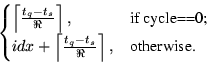
i) LBSearch: S starts out by setting the lower bound :

idx_lb(t_q, t_s) = $\begin{displaymath}\begin{cases}\left\lceil \frac{t_q-t_s}{\Re} \right\rceil, ... ...rac{t_q-t_s}{\Re} \right\rceil, & \text{otherwise.} \end{cases}\end{displaymath}$

where idx is the address of the last written page and $\Re$ a constant indicating the maximum number of data records per page. It then deploys the LBSearch(ts, idx_lb) procedure as illustrated in Algorithm 2. It is easy to see that in each recursion step, LBSearch always moves clockwise (increasing time order) and that idx_lb $\leq$ idx_{t_q}.

$\begin{algorithm} % latex2html id marker 324 [h] \begin{small} \caption{LBSearch... ...t_q, t_2));$\par\EndIf \EndProcedure \end{algorithmic}\end{small}\end{algorithm}$

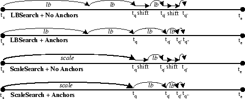
Figure 4: Searching By Timestamp. t_s: oldest timestamp on flash (t_e: newest), t_q: the query (timestamp), lb: The lower bound obtained using either idx_lb or idx_scaled.

$\epsfbox{figs/searching.eps}$

It is important to note that a lower bound can only be estimated if the fetched page, on each step of the recursion, contains a timestamp value. Our discussion so far, assumes that the only pages that carry a timestamp are data pages which contain a sequence of data records {[ts₁, val₁]...[ts₁, val]}. In such a case, the LBSearch has to shift right until a data page is located. In our experiments we noted that this deficiency could add in some cases 3-4 additional page reads. In order to correct the problem we store the last known timestamp inside each index page (named Anchor).

ii) ScaleSearch: When index pages are uniformly spread out across the flash media, then a more aggressive search strategy might be more effective. In ScaleSearch, which is the technique we deployed in MicroHash, instead of using idx_lb in the first step we use idx_scaled:

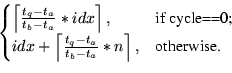
idx_scaled(t_q, t_s) = $\begin{displaymath}\begin{cases}\left\lceil \frac{t_q-t_a}{t_b-t_a}*idx \right... ...q-t_a}{t_b-t_a}*n \right\rceil, & \text{otherwise.} \end{cases}\end{displaymath}$

We then use LBSearch in order to refine the search. Note that idx_scaled might in fact be larger than idx_{t_q} in which case LBSearch might need to move counter-clockwise (decreasing time order).

Performing a timestamp-based range query Q(t_q, a, b) is a simple extension of the equality search. More specifically, we first perform a ScaleSearch for the upper bound b (i.e. Q(t_q, b)) and then sequentially read backwards until a is found. Note that data pages are chained in reverse chronological order (i.e. each data page maintains the address of the previous data page) and therefore this operation is very simple.

6.3 Search Optimizations

In the basic MicroHash approach, index pages on flash might not be fully occupied. This incurs a significant performance penalty when somebody performs a search by value, because the system has to read in memory more pages than necessary. In this section we present two alternative methods that alleviate this performance penalty. The first method, named Elf-Like Chaining (ELC), eliminates non-full index pages which as a result decreases the number of pages required to answer a query, while the second method, named Two-Phase Read minimizes the number of bytes transferred from the flash media.

6.3.1 Elf-Like Chaining (ELC)

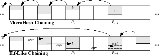
In the MicroHash index, pages are chained using a back-pointer as illustrated in Figure 5 (named MicroHash Chaining). Inspired from the update policy of the ELF filesystem [2], we also investigate, and later experimentally evaluate, the Elf-like Chaining (ELC) mechanism. The objective of ELC is to create a linked list in which each node, other than the last node, is completely full. This is achieved by copying the last non-full index page into a newer page, when new index records are requested to be added to the index. This procedure continues until an index page becomes full, at which point it is not further updated.

Figure 5: Index Chaining Methods: a) MicroHash Chaining and b) ELF-like Chaining.

$\epsfbox{figs/elf.eps}$

To better understand the two techniques, consider the following scenario (see Figure 5): An index page on flash (denoted as p_i (i $\leq$ n)), contains k ( k < p^size_i) index records {ir₁, ir₂,..., ir_k} that in our scenario map to directory bucket v. Suppose that we create a new data page on flash at position p_i+1. This triggers the creation of l additional index records, which in our scenario map to the same bucket v. In MicroHash Chaining (MHC), the buffer manager simply allocates a new index page for v and keeps the sequence {ir₁, ir₂,..., ir_l} in memory until the LRU replacement policy forces the page to be written out. Assuming that the new index sequence is forced out of memory at p_i+3, then p_i will be back-pointed by p_i+3 as shown in Figure 5. In Elf-Like Chaining (ELC), the buffer manager reads p_i in memory and then augments it with the l new index records (i.e. {ir₁,..., ir_k,..., ir_l+k}). However, p_i is not updated due to the write and wear constraint, but instead the buffer manager writes the new l + k sequence to the end of the flash media (i.e. at p_i+3). Note that p_i is now not backpointed by any other page and will not be utilized until the block delete, guided by the idx pointer, erases it.

The optimal compaction degree of index pages in ELC significantly improves the search performance of an index as it is not required to iterate over partially full index pages. However, in the worse case, ELC might introduce an additional page read per indexed data record. Additionally we observed in our experiments, presented in Section 8, that ELC requires on average 15% more space than the typical MicroHash chaining. In the worst case, the space requirement of ELC might double the requirement of MHC.

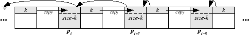
Figure 6: Sequential Trashing in ELC.

$\epsfbox{figs/elf2.eps}$

Consider again the scenario under discussion. This time assume that the buffer manager reads p_i in memory and then augments p^size_i (a full page) new index records as shown in Figure 6. That will evict p_i to some new address (in our scenario p_i+3). However some additional p^size_i - k records are still in the buffer. Assume that these pages are at some point evicted from memory to some new flash position (in our scenario p_i+5). So far we utilized three pages (p_i, p_i+3 and p_i+5) while the index records could fit into only 2 index pages (i.e. k + p^size_i records, k < p^size_i). When the same scenario is repeated, then we say that ELC suffers from Sequential Trashing and ELC will require double the required space to accommodate all index records.

6.3.2 Two-Phase Page Reads

Our discussion so far assumes that pages are read from the flash media on a page-by-page basis (usually 512B per page). When pages are not fully occupied, such as index pages, then a lot of empty bytes (padding) is transferred from the flash media to memory. In order to alleviate this burden, in [1] we exploit the fact that reading from flash can be performed at any granularity (i.e. as small as a single byte). Specifically, we propose the deployment of a Two-Phase Page Read in which the MCU reads a fixed header from flash in the first phase, and then reads the exact amount of bytes in the next phase. We experimentally evaluated the performance of two-phase reads versus single phase reads using the RISE sensor node and found that such an approach significantly minimizes energy consumption.

7 Experimental Methodology

In this section we describe the details of our experimental methodology.

7.1 Experimental Testbed

We have implemented MicroHash along with a tiny LRU BufferManager in nesC[6], the programming language of TinyOS[7]. TinyOS is an open-source operating system designed for wireless embedded sensor nodes. It was initially developed at UC-Berkeley and has been deployed successfully on a wide range of sensors including the RISE mote. TinyOS uses a component-based architecture that enables programmers to wire together in on-demand basis the minimum required components. This minimizes the final code size and energy consumption as sensor nodes are extremely power and memory limited. nesC [6] is the programming language of TinyOS and it realizes its structuring concepts and its execution model.

Our implementation consists of approximately 5000 lines of code and requires at least 3KB in SRAM. Specifically we use one page as a write buffer, two pages for reading (i.e. one for an index page and one for a data page), one page as an indexing buffer, one for the directory and one final page for the root page. In order to increase insertion performance and index page compactness, we also supplement additional index buffers (i.e. 2.5KB-5KB).

We had to write a library that simulates the flash media using an operating system file, in order to run our code in TOSSIM [8], the simulation environment of TinyOS. We additionally wrote a library that intercepts all messages communicated from TinyOS to the flash library and prints out various statistics and one final library that visualizes the flash media using bitmap representations.

7.2 PowerTOSSIM - Energy Modeling

PowerTOSSIM is a power modeling extension to TOSSIM presented in [14]. In order to simulate the energy behavior of the RISE sensor we extended PowerTOSSIM and added annotations to the MicroHash structure that accurately provide information when the power states change in our environment. We have focused our attention on precisely capturing the flash performance characteristics as opposed to capturing the precise performance of other less frequently used modules (the radio stack, on-chip flash, etc).

Our power model follows our detailed measurements of the RISE platform [1], which are summarized as following: We use a 14.8 MHz 8051 core operating at 3.3V with the following current consumption 14.8mA (On), 8.2mA (Idle), 0.2 $\mu$ A (Off). We utilize a 128MB flash media with a page size of 512B and a block size of 16KB. The current to read, write and block delete was 1.17mA, 37mA and 57 $\mu$ A and the time to read in the three pre-mentioned states was 6.25ms, 6.25ms, 2.27ms.

Using these parameters, we performed an extensive empirical evaluation of our power model and found that PowerTOSSIM is indeed a very useful and quite accurate tool for modeling energy in a simulation environment. For example we measured the energy required to store 1 MB of raw data on an RISE mote and found that this operation requires 1526mJ while the same operation in our simulation environment returned 1459mJ, which has a error of only 5%. On average we found that PowerTOSSIM provided an accuracy of 92%.

7.3 Dataset Descriptions

Since we cannot measure environmental conditions, such as temperature or humidity in a simulation environment, we adopt a trace-driven experimental methodology in which a real dataset is fed into the TOSSIM simulator. More specifically, we use the following datasets:

Washington State Climate: This is a real dataset of atmospheric data collected by the Department of Atmospheric Sciences at the University of Washington [21]. Our 268MB dataset contains readings on a minute basis between January 2000 and February 2005. The readings, which are recorded at a weather logging station in Washington, include barometric pressure, wind speed, relative humidity, cumulative rain and others. Since many of these readings are not typically measured by sensor nodes we only index the temperature and pressure readings, and use the rest readings as part of the data included in a record. Note that this is a realistic assumption, as sensor nodes may concurrently measure a number of different parameters.

Great Duck Island (GDI 2002): This is a real dataset from the habitat monitoring project on the Great Duck Island in Maine [15]. We use readings from one of the 32 nodes that were used in the spring 2002 deployment, which included the following readings: light, temperature, thermopile, thermistor, humidity and voltage. Our dataset includes approximately 97,000 readings that were recorded between October and November 2002.

8 Experimental Evaluation

In this section we present extensive experiments to demonstrate the performance effectiveness of the MicroHash Index structure. The experimental evaluation described in this section focuses on three parameters: i) Space Overhead, of maintaining the additional index pages, ii) Search Performance, which is defined as the average number of pages accessed for finding the required record and iii) Energy Consumption, for indexing the data records. Due to the design of the MicroHash index, each page was written exactly once during a cycle. Therefore there was no need to experimentally evaluate the wear-leveling performance.

8.1 Overhead of Index Pages

In the first series of experiments we investigate the overhead of maintaining the additional index pages on the flash media. For this reason we define the overhead ratio $\Phi$ as follows: $\Phi$ = ${\frac{{Index Pages}}{{Data Pages + Index Pages}}}$ . We investigate the parameter $\Phi$ using a) An increasing buffer size and b) An increasing data record size.

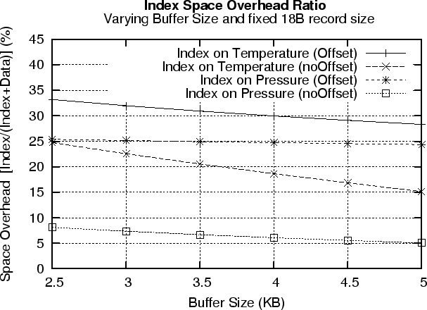
We also evaluate two different index record layouts: a) Offset, in which an index record has the following form {pageid,offset} and NoOffset, in which an index record has the form {pageid}. We use the five year timeseries from the Washington state climate dataset and index data records based on their temperature and pressure attribute. The data record on each of the 2.9M time instances was 18 bytes (i.e. 8B timestamp + 5x2B readings).

Figure 7: Space Overhead of Index Pages with a) varying buffer size and b) varying record size.

$\epsfbox{figs/space-overhead-buffer.eps}$

$\epsfbox{figs/space-overhead-recordsize.eps}$

8.1.1 Increasing Buffer Size

Figure 7 (top) presents our results using a varying buffer. The figure shows that in all cases a larger buffer helps in fitting more index records per page which therefore also linearly reduces the overall space overhead. In both the pressure and temperature case, the noOffset index record layout significantly reduces the space overhead as less information is required to be stored inside an index record.

The figure shows that indexing on pressure achieves a lower overhead. This is attributed to the fact that the pressure changes slower than the temperature over time. This leads to fewer evictions of index pages during the indexing phase which consequently also increases the index page occupancy. We found that a 3KB buffer suffices to achieve occupancy of 75-80% in index pages.

8.1.2 Increasing Data Record Size

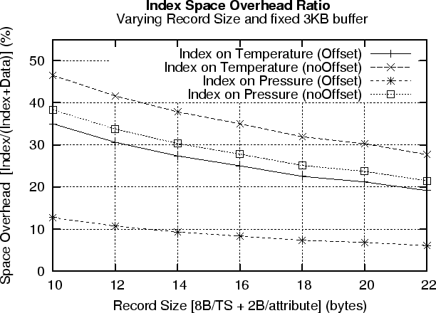
Sensor nodes usually deploy a wide array of sensors, such as a photo sensor, magnetometer, accelerometer and others. Therefore the data record size on each time instance might be larger than the minimum 10B size (8B timestamp and 2B data value). Figure 7 (bottom) presents our results using a varying data record size. The figure shows that in all cases a larger data record size decreases the space overhead proportion. Therefore it does not become more expensive to store the larger data records on flash.

8.2 Searching By Timestamp

In the next experimental series, we investigate the average number of pages that must be read in order to find a record by its timestamp. We search for 100 timestamps selected uniformly at random, from the available five year range, and then calculate the average number of pages read. Note that if we did not use an index, and thus had only data records on the flash, then we could find the expected record in O(1) time as we could manipulate the position of the record directly. However, this would also violate our wear leveling mechanism.

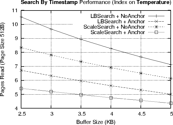
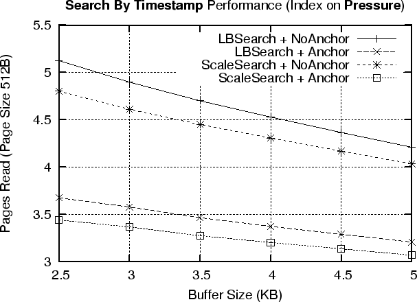
We evaluate the proposed search by timestamp methods LBSearch and ScaleSearch under two different index page layouts: a) Anchor, in which every index page stores the last known data record timestamp and b) NoAnchor, in which an index page does not contain any timestamp information.

Figure 8 shows our results using the Washington state climate dataset for both an index on Temperature (Figure 8 top) and an Index on Pressure (Figure 8 bottom). The figures show that using an anchor inside an index pages is a good choice as it usually reduces the number of page reads by two, while it does not present a significant space overhead (only 8 additional bytes). The figures also show that ScaleSearch is superior to LBSearch as it exploits the uniform distribution of index pages on the flash media. This allows ScaleSearch to get closer to the result, in the first step of the algorithm.

The figures finally show that even though the time window of the query is quite large (i.e. 5 years or 128MB), ScaleSearch is able to find a record by its timestamp in approximately 3.5-5 page reads. Given that a page read takes 6.25ms, this operation requires according to the RISE model only 22-32ms or 84-120 $\mu$ J.

Figure 8: Search-By-Timestamp Performance of the MicroHash Index.

$\epsfbox{figs/ts_search_temp.eps}$ $\epsfbox{figs/ts_search_pressure.eps}$

8.3 Searching by Value: MicroHash Chaining vs. ELF-Like Chaining

The cost of searching a particular value on the flash media is linear with respect to the size of the flash media. However, a simple linear scan over 256 thousands pages found on a 128MB flash media, would result in an overwhelming large search cost. One factor that significantly affects search performance is the occupancy of index pages. In the basic MicroHash approach, index pages on the flash might not be fully occupied. If index pages are not fully utilized, then a search would require iterating over more pages than necessary.

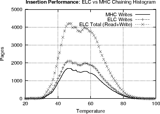
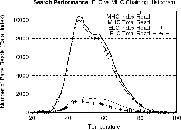
In this section we perform an experimental comparison of the index chaining strategies presented in Section 6.3. We evaluate both MicroHash Chaining (MHC) and Elf-like chaining (ELC) using a fixed 3KB buffer. We deploy the chaining methods when the temperature is utilized as the index (we obtained similar results for pressure). Our evaluation parameters are : a) Indexing Performance (pages written) and b) Search Performance (pages read).

Figure 9: Comparing MicroHash Chaining (MHC) with ELF-like Chaining (ELC) using a) Insertion Performance and b) Searching Performance by Value.

$\epsfbox{figs/elf-indexing.eps}$

$\epsfbox{figs/elf-searching.eps}$

Figure 9 (top) shows that MHC always requires less page writes than ELC. The reason is that ELC's strategy results in about 15% sequential trashing, which is the characteristic presented in Section 6.3. Additionally, ELC requires a large number of page reads in order to replicate some of the index records. This is presented in the ELC Total plot, which essentially shows that it requires as many page reads as page writes in order to index all records. On the other hand, ELC's strategy results in linked lists of fully occupied index pages than MHC. This has as a result, an improved search performance since the system is required to fetch less index pages during search. This can be observed in Figure 9 (bottom), in which we present the number of index pages read and the total number of pages (index + data). On the other hand, we also observe that ELC only reduces the overall read gain to about 10%. This happens because the reading of data page, dominates the overall reading cost. However when searches are more frequent, then the 10% is still an advantage and therefore ELC is more appropriate than its counterpart MHC.

8.4 Great Duck Island Trace

In this last experimental series we index measurements from the great duck island study, described in Section 7.3. For this study we allocate a fixed 3KB index buffer along with a 4MB flash media that has adequate space to store all the 97,000 20-byte data readings.

In each run, we index on a specific attribute (i.e. Light, Temperature, Thermopile, Thermistor, Humidity and Voltage). We then record the overhead ratio of index pages $\Phi$ , the energy required by the flash media to construct the index as well as the average number of page reads that were required to find a record by its timestamp. We omit the search by value results, due to lack of space, but the results are very similar to those presented in the previous subsection.

Table 2 shows that the index pages never require more that 30% more space on the flash media. For some readings that do not change frequently (e.g. humidity), we observe that the overhead is as low as 8%. The table also shows that indexing the records has only a small increase in energy demand. Specifically, the energy cost of storing the records on flash without an index was 3042mJ, which is on average only 779mJ less than using an index. Therefore maintaining the index records does not impose a large energy overhead. Finally the table shows that we were able to find any record by its timestamp with 4.75 page reads on average.

Table: Performance Results from Indexing and Searching the Great Duck Island dataset.

Index On	Overhead	Energy	ScaleSearch
Attribute	Ratio $\Phi$ %	Index (mJ)	Page Reads
Light	26.47	4,134	4.45
Temperature	27.14	4,172	5.45
Thermopile	24.08	4,005	6.29
Thermistor	14.43	3,554	5.10
Humidity	7.604	3,292	2.97
Voltage	20.27	3,771	4.21

9 Related Work

There has been a lot of work in the area of query processing, in-network aggregation and data-centric storage in sensor networks. To the best of our knowledge, our work is the first that addresses the indexing problem on sensor nodes with flash memories.

A large number of flash-based file systems have been proposed in the last few years, including the Linux compatible Journaling Flash File System (JFFS and JFFS2)[17], the Virtual File Allocation Table (VFAT) for Windows compatible devices and the Yet Another Flash File System (YAFFS)[18], specifically designed for NAND flash with it being portable under Linux, uClinux, and Windows CE. The first file system for sensor nodes was Matchbox and this is provided as an integral part of the TinyOS [7] distribution. Recently the Efficient Log Structured Flash File System (ELF)[2] shows that it offers several advantages over Matchbox including higher read throughput and random access by timestamp. Other filesystems for embedded microcontrollers that utilize flash as a storage medium include the Transactional Flash File System (TFFS) [5]. However the main job of a file system is to organize the blocks of the storage media into files and directories and to provide transaction semantics on these attributes. Therefore a filesystem does not support the retrieval of records by their value as we do in our approach.

An R-tree and B-Tree index structure for flash memory on portable devices, such as PDA's and cell phones, has been proposed in [22] and [23] respectively. These structures use an in-memory address translation table, which hides the details of wear-leveling mechanism. However, such a structure has a very large footprint (3-4MB) which constitutes it inapplicable in the context of microcontrollers with limited SRAM.

Wear-Leveling techniques have also been reported by flash card vendors such as Sandisk [20]. These techniques are executed by a microcontroller which is located inside the flash card. The Wear-Leveling techniques are only executed within 4MB zones and are thus local rather than global which is the case in MicroHash. A main drawback of the local wear-leveling techniques is that the writes are no longer spread out uniformly across all available pages. Finally these techniques assume a dedicated controller while our techniques can be executed by the microcontroller of the sensor device.

Systems such as TinyDB[11] and Cougar[16] are optimized for sensor nodes with limited storage and relatively shorter-epochs, while our techniques are designated for sensors with larger external flash memories and longer epochs. Note that in TinyDB users are allowed to define fixed size materialization points through the STORAGE POINT clause. This allows each sensor to gather locally in a buffer some readings, which cannot be utilized until the materialization point is created in its entirety. Therefore even if there was enough storage to store MBs of data, the absence of efficient access methods makes the retrieval of the desired values expensive.

10 Conclusions

In this paper we propose the MicroHash index which is an efficient external memory hash index that addresses the distinct characteristics of flash memory. We also provide an extensive study of NAND flash memory when this is used as a storage media of a sensor device. Our design can serve several applications, including sensor and vehicular networks, which generate temporal data and utilize flash as the storage medium. We expect that our proposed access method will provide a powerful new framework to cope with new types of queries, such as temporal or top-k, that have not been addressed adequately to this date. Our experimental evaluation with real traces from environmental and habitant monitoring show that the structure we propose is both efficient and practical.

Acknowledgements

We would like to thank Joe Polastre (UC Berkeley) for providing us the Great Duck Island data trace and Victor Shnayder (Harvard) for his help on the PowerTOSSIM environment. We would also like to thank Abhishek Mitra and Anirban Banerjee (UC Riverside) for their assistance in the RISE micro-benchmarks. Finally, we would like to thank our shepherd, Andrea Arpaci-Dusseau, and the anonymous reviewers for their numerous helpful comments. This work was supported by grants from NSF ITR #0220148, #0330481.

Bibliography

1: Banerjee A., Mitra A., Najjar W., Zeinalipour-Yazti D., Kalogeraki V. and Gunopulos D.,
``RISE Co-S : High Performance Sensor Storage and Co-Processing Architecture'',
In IEEE SECON, Santa Clara, CA, USA, to appear in 2005.
2: Dai H., Neufeld M., Han R.,
``ELF: an efficient log-structured flash file system for micro sensor nodes'',
In SenSys, Baltimore, pp. 176-187, 2004.
3: Dipert B., Levy M.,
``Designing with Flash Memory'',
AnnaBooks Publisher, 1994.
4: Fagin R., Nievergelt J., Pippenger N., Strong H.R.:
``Extendible Hashing - A Fast Access Method for Dynamic Files'',
In ACM TODS, vol 4(3), pp. 315-344, 1979.
5: Gal E. and Toledo S.,
``A Transactional Flash File System for Microcontrollers'',
In USENIX 2005, Anaheim, CA, pp. 89-104, 2005.
6: Gay D., Levis P., Von Behren R. Welsh M., Brewer E. and Culler D.,
``The nesC Language: A Holistic Approach to Networked Embedded Systems'',
In ACM PLDI, San Diego, pp. 1-11, 2003.
7: Hill J., Szewczyk R., Woo A., Hollar S., Culler D., Pister K..
``System Architecture Directions for Networked Sensors'',
In ASPLOS, Cambridge, MA, pp. 93-104, 2000.
8: Levis P., Lee N., Welsh M., and Culler D.,
``TOSSIM: Accurate and Scalable Simulation of Entire TinyOS Applications'',
In ACM SenSys, Los Angeles, CA, 2003.
9: Litwin W.,
``Linear Hashing: A New Tool for File and Table Addressing'',
VLDB 1980: 212-223.
10: Lymberopoulos D., Savvides A.,
``XYZ: A Motion-Enabled, Power Aware Sensor Node Platform for Distributed Sensor Network Applications'',
In IPSN, Los Angeles, pp. 449-454, 2005.
11: Madden S.R., Franklin M.J., Hellerstein J.M., Hong W.,
"The Design of an Acquisitional Query Processor for Sensor Networks",
In ACM SIGMOD, San Diego, CA, USA, pp. 491-502, 2003.
12: Madden S.R., Franklin M.J., Hellerstein J.M., Hong W.,
``TAG: a Tiny AGgregation Service for Ad-Hoc Sensor Networks'',
In OSDI, Boston, MA, pp. 131-146, 2002.
13: Sadler C., Zhang P., Martonosi M., Lyon S.,
``Hardware Design Experiences in ZebraNet'',
In ACM SenSys, Baltimore, pp. 227-238, 2004.
14: Shnayder V., Hempstead M., Chen B., Werner-Allen G., and Welsh M.,
``Simulating the Power Consumption of Large-Scale Sensor Network Applications'',
In ACM SenSys, pp. 188-200, 2004.
15: Szewczyk R., Mainwaring A., Polastre J., Anderson J., Culler D.,
``An Analysis of a Large Scale Habitat Monitoring Application'',
In ACM SenSys, Baltimore, MD, pp. 214-226, 2004.
16: Yao Y., Gehrke J.E.,
"Query Processing in Sensor Networks",
In CIDR, Asilomar, CA, USA, 2003.
17: Woodhouse D.
``JFFS : The Journalling Flash File System''
Red Hat Inc., Available at: https://sources.redhat.com/jffs2/jffs2.pdf
18: Wookey
``YAFFS - A filesystem designed for NAND flash'',
Linux 2004 Leeds, U.K.
19: Ramakrishnan R., Gehrke J.,
Database Management Systems,
McGraw-Hill, Third edition, 2002.
20: ``Sandisk Flash Memory Cards - Wear Leveling'',
October 2003 White Paper,
Available at: https://sandisk.com/pdf/oem/ WPaperWearLevelv1.0.pdf
21: Live From Earth and Mars Project
University of Washington, Seattle https://www-k12.atmos.washington.edu/k12/grayskies/
22: Wu C-H., Chang L-P., Kuo T-W.,
``An Efficient R-tree Implementation Over Flash-Memory Storage Systems'',
In RTCSA, Taiwan, pp. 409-430, 2003.
23: Wu C-H., Chang L-P., Kuo T-W.,
``An Efficient B-Tree Layer for Flash Memory Storage Systems'',
In RTCSA, New Orleans, pp. 17-24, 2003.
24: Xu N., Rangwala S., Chintalapudi K., Ganesan D., Broad A., Govindan R. and Estrin D.,
``A Wireless Sensor Network for Structural Monitoring'',
In Sensys, Baltimore, MD, pp. 13-24, 2004.

Need help?

Last changed: 16 Nov. 2005 jel

MicroHash: An Efficient Index Structure for Flash-Based Sensor Devices