We survey, evaluate, and compare a variety of approaches to the variable-sized precinct auditing problem, including the SAFE method [11] which is based on theory developed for equal-sized precincts. We introduce new methods such as the negative-exponential method ``NEGEXP'' that select precincts independently for auditing with predetermined probabilities, and the ``PPEBWR'' method that uses a sequence of rounds to select precincts with replacement according to some predetermined probability distribution that may depend on error bounds for each precinct (hence the name PPEBWR: probability proportional to error bounds, with replacement), where the error bounds may depend on the sizes of the precincts, or on how the votes were cast in each precinct.
We give experimental results showing that NEGEXP and PPEBWR can dramatically reduce (by a factor or two or three) the cost of auditing compared to methods such as SAFE that depend on the use of uniform sampling. Sampling so that larger precincts are audited with appropriately larger probability can yield large reductions in expected number of votes counted in an audit.
We also present the optimal auditing strategy, which is nicely representable as a linear programming problem but only efficiently computable for small elections (fewer than a dozen precincts). We conclude with some recommendations for practice.
Post-election audits are an essential tool for ensuring the integrity of election outcomes. They can detect, with high probability, both errors due to machine mis-programming and errors due to malicious manipulation of electronic vote totals. By using statistical samples, they are quite efficient and economical. This paper explores auditing approaches that achieve improved efficiency (sometimes by a factor of two or three, measured in terms of the number of votes counted) over previous methods.
Suppose we have an election with ![]() precincts,
precincts, ![]() , ...,
, ...,
![]() . Let
. Let ![]() denote the number of voters who voted in precinct
denote the number of voters who voted in precinct
![]() ; we call
; we call ![]() the ``size'' of the precinct
the ``size'' of the precinct ![]() . Let the total
number of such voters be
. Let the total
number of such voters be ![]() . Assume without loss of
generality that
. Assume without loss of
generality that
![]() .
.
We focus on auditing precincts as opposed to votes because this is the common form of auditing encountered in practice. If one is interested in sampling votes, then the results in Aslam et al. [1] apply because the votes can be modeled as precincts of equal size (in particular, of size one). In this paper, we are interested in the more general problem, that is, when precincts have different sizes.
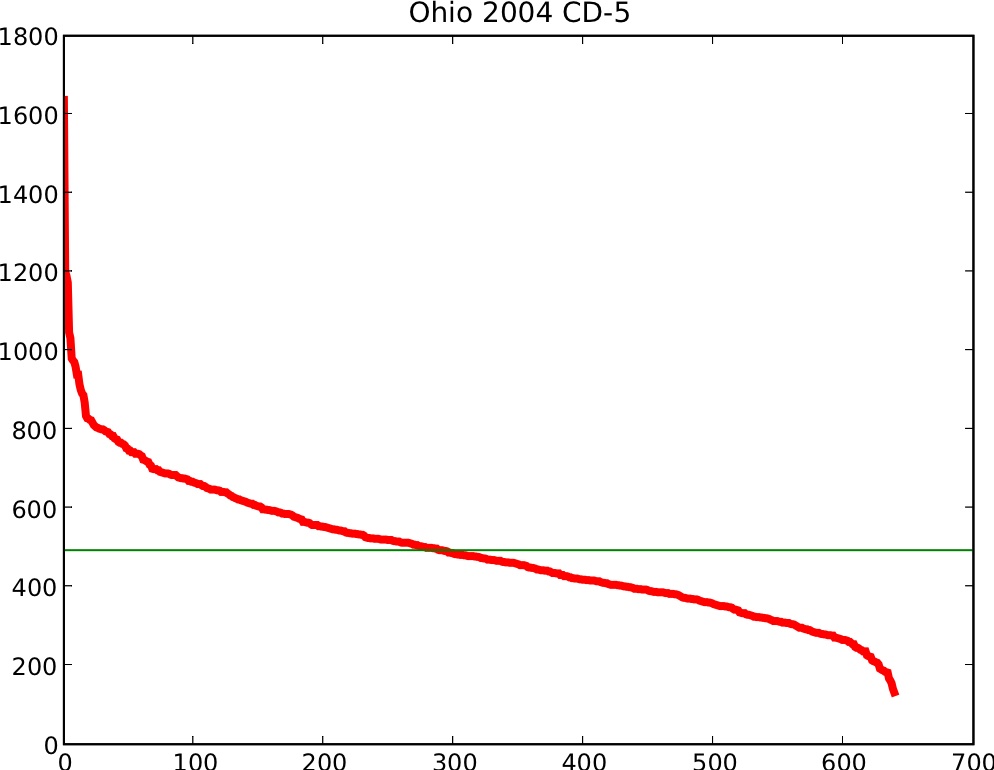
Precinct sizes can vary dramatically, sometimes by an order of magnitude or more. See Figure 2.
Methods for auditing elections must, if they are to be efficient and effective, take such precinct size variations into account.
Suppose further that in precinct ![]() we have both electronic records
and paper records for each voter. The electronic records are easy to
tally. For the purposes of this paper, the paper records are used only as a
source of authoritative information when the electronic records are
audited. They may be considered more authoritative since the voters
may have verified them directly. In practice, more care is needed,
since the electronic records could reasonably be judged as more
authoritative in situations where the paper records were obviously
damaged or lost and the electronic records appear undamaged.
we have both electronic records
and paper records for each voter. The electronic records are easy to
tally. For the purposes of this paper, the paper records are used only as a
source of authoritative information when the electronic records are
audited. They may be considered more authoritative since the voters
may have verified them directly. In practice, more care is needed,
since the electronic records could reasonably be judged as more
authoritative in situations where the paper records were obviously
damaged or lost and the electronic records appear undamaged.
Auditing is desirable since a malicious party, the ``adversary,'' may have manipulated some of the electronic tallies so that a favored candidate appears to have won the election. It is also possible for a simple software bug caused the electronic tallies to be inaccurate. However, we focus on detecting malicious adversarial behavior because it is the more challenging task.
A precinct can be ``audited'' by re-counting by hand the paper records of that precinct to confirm that they match the electronic totals for that precinct. We ignore here the important fact that hand-counting may be inaccurate, and assume that any discrepancies are due to fraud on the part of the adversary. In practice, the discrepancy might have to be larger than some prespecified threshold to trigger a conclusion of fraud in that precinct.
See the overviews [8,13,6] for information about current election auditing procedures. In this paper we ignore many of the complexities of real elections; these complexities are addressed in other papers. We do so in order to focus on our central issue: how to select a sample of precincts to audit when the precincts have different sizes. See Neff [12], Cordero et al. [5], Saltman [17], Dopp et al. [7], and Aslam et al. [1], for additional discussion of the mathematics of auditing, and additional references to the literature.
We begin with an overview of the auditor's general approach in Section 2. In Section 3 we review the adversary's objectives and capabilities. Section 4 then reviews the auditor's strategy. Some known results for auditing when all precincts have equal size are discussed in Section 5. We next review in Section 6 the ``SAFE'' method, which deals with variable-sized precincts using the mathematics developed for equal-sized precincts, by first deriving a lower bound on the number of precincts that must have been corrupted, if the election outcome was changed. Section 7 introduces basic auditing methods, where each precinct is chosen independently according to a precomputed probability distribution. A particularly attractive basic auditing method is introduced in Section 8; this method is called the ``negative-exponential'' (NEGEXP) auditing method. We then consider audits where precincts are not chosen independently. Section 9 introduces the method of sampling with probability proportional to error bounds, with replacement (PPEBWR); a special case of this procedure is PPSWR, ``sampling with probability proportional to size, with replacement.'' Section 10 discusses vote-dependent auditing, where the probability of auditing a precinct depends on the actual vote counts for each candidate. Section 11 gives experimental results using data from Ohio and Minnesota. Section 12 presents a method based on linear programming for determining an optimal auditing procedure, which unfortunately appears to be computationally too expensive for practical use. Section 13 closes with discussion and recommendations for practice.
We assume here that the election is a winner-take-all (plurality)
election from a field of ![]() candidates.
candidates.
After the election, the auditor randomly selects a sample of precincts for the post-election audit. In each selected precinct the paper ballots are counted by hand; the totals obtained in this manner are then compared with the electronic tallies. We assume that the paper ballots are maintained securely and that they can be accurately counted during the post-election audit.
The auditor wishes to assure himself (and everyone else) that the level of error and/or fraud in the election is likely to be low or nonexistent, or at least insufficient to have changed the election outcome. If the audit finds no (significant) discrepancies between the electronic and paper tallies, the auditor announces that no fraud was discovered, and the election results may be certified by the appropriate election official.
However, if significant discrepancies are found between the electronic and paper tallies, additional investigations may be appropriate. For example, state law may require a full recount of the paper ballots. Stark [19] gives procedures for incrementally auditing larger and larger samples when discrepancies are found, until the desired level of confidence in the election outcome is achieved.
When planning the audit, the auditor knows the number ![]() of reported (electronic)
votes for each candidate
of reported (electronic)
votes for each candidate ![]() in precinct
in precinct ![]() , and
the total size
, and
the total size ![]() (total number of votes cast) of each
precinct
(total number of votes cast) of each
precinct ![]() . The auditor also knows the reported margin of victory, denoted
. The auditor also knows the reported margin of victory, denoted
![]() of the winning candidate over the runner-up--this is the
difference between the number of votes reported for the apparently
victorious candidate and the number of votes reported for the
runner-up. Larger audits are appropriate when the margins of victory
are smaller (see, e.g., Norden et al. [13]).
of the winning candidate over the runner-up--this is the
difference between the number of votes reported for the apparently
victorious candidate and the number of votes reported for the
runner-up. Larger audits are appropriate when the margins of victory
are smaller (see, e.g., Norden et al. [13]).
We believe that the audit should be designed to achieve a pre-specified level of confidence in the election outcome, i.e., when an election is ultimately certified, one should be confident, in a statistically quantifiable manner, that the election outcome is correct. It is the correct (and efficient) approach. Naive methods that audit a fixed fraction of precincts tend to waste money when the margin of victory is large, and provide poor confidence in the election outcome when the margin of victory is small. See McCarthy et al. [11].
In order to ensure that an election outcome is correct, one must
be able to detect levels of fraud sufficient to change the outcome
of the election.
We thus assume the auditor desires to test at a certain
significance level ![]() that error or fraud is unlikely to have affected
the election outcome. A well-designed audit can reduce the likelihood
that significant fraud or error has gone undetected. A significance
level of
that error or fraud is unlikely to have affected
the election outcome. A well-designed audit can reduce the likelihood
that significant fraud or error has gone undetected. A significance
level of ![]() means that the chance that error large enough
to have changed the election outcome will go undetected is one in
twenty.
means that the chance that error large enough
to have changed the election outcome will go undetected is one in
twenty.
Let ![]() denote the ``confidence level'' of the audit, where
denote the ``confidence level'' of the audit, where
![]() Thus, a test at significance level
Thus, a test at significance level ![]() provides a confidence level
of
provides a confidence level
of ![]() . This is independent of the way fraud was
committed (at the level of the machine, precinct, vote or other) because we only model the overall fraud in our formulas.
We follow Stark [19] in adopting as our null hypothesis
``the (electronic) election outcome is incorrect'', so that
. This is independent of the way fraud was
committed (at the level of the machine, precinct, vote or other) because we only model the overall fraud in our formulas.
We follow Stark [19] in adopting as our null hypothesis
``the (electronic) election outcome is incorrect'', so that ![]() is an upper bound on the probability that the null hypothesis will be
rejected (i.e. that the electronic outcome will be accepted) when the
null hypothesis is true (the electronic outcome is wrong).
is an upper bound on the probability that the null hypothesis will be
rejected (i.e. that the electronic outcome will be accepted) when the
null hypothesis is true (the electronic outcome is wrong).
Depending on the precinct sizes, the reported votes for each candidate, and thus the reported margin of victory, the auditor determines how to select an appropriately-sized random sample of precincts for auditing.
We explore three methods by which the auditor chooses a sample:
If all precincts have the same size, one may measure the cost of performing an audit in terms of the (expected) number of precincts audited. If precincts have a variety of sizes, the (expected) number of votes counted appears to be a better measure of auditing cost. The auditing cost is most reasonably measured in person-hours, which will be proportional to the number of votes recounted. The overall cost may have a constant additive term for each precinct (a setup cost), but this should be small compared to the cost to audit the votes.
We assume the adversary wishes to corrupt enough of the electronic
tallies so that his favored candidate
wins the most votes according to the reported electronic tallies.
Without loss
of generality, we'll let candidate ![]() be the adversary's favored
candidate. The adversary tries to do his manipulations in such a way as to
minimize the chance that his changes to the electronic tallies
will be caught during the post-election audit.
be the adversary's favored
candidate. The adversary tries to do his manipulations in such a way as to
minimize the chance that his changes to the electronic tallies
will be caught during the post-election audit.
Let ![]() denote the actual number of (paper) votes for
candidate
denote the actual number of (paper) votes for
candidate ![]() in precinct
in precinct ![]() , and let
, and let ![]() denote the
reported number of (electronic) votes for candidate
denote the
reported number of (electronic) votes for candidate ![]() in
precinct
in
precinct ![]() . With no adversarial manipulation, we will have
. With no adversarial manipulation, we will have
![]() for all
for all ![]() and
and ![]() . We ignore in this paper small explainable
discrepancies that can be handled by slight modifications to the
procedures discussed here.
. We ignore in this paper small explainable
discrepancies that can be handled by slight modifications to the
procedures discussed here.
We thus have for all ![]() :
:
![]() the total number of paper votes cast in precinct
the total number of paper votes cast in precinct ![]() is equal to the
number of electronic votes cast in precinct
is equal to the
number of electronic votes cast in precinct ![]() ; this number is
; this number is ![]() ,
the ``size'' of precinct
,
the ``size'' of precinct ![]() . (Our techniques can perhaps be extended to handle
situations where such reconciliation is not done; we have not yet examined
this question closely.)
. (Our techniques can perhaps be extended to handle
situations where such reconciliation is not done; we have not yet examined
this question closely.)
Let ![]() denote the total actual number of votes for candidate
denote the total actual number of votes for candidate ![]() :
:
![]() and let
and let ![]() denote the total number of votes reported for candidate
denote the total number of votes reported for candidate ![]() :
:
![]() The adversary's favored candidate, candidate
The adversary's favored candidate, candidate ![]() , will be the
winner of the electronic report totals if
, will be the
winner of the electronic report totals if
![]()
We assume for now that the election is really between candidate ![]() and candidate
and candidate ![]() , so that the adversary's objective is to ensure that
candidate
, so that the adversary's objective is to ensure that
candidate ![]() is reported to win the election and that candidate
is reported to win the election and that candidate ![]() is not.
There may be other candidates in the race, but for the moment we'll
assume that they are minor candidates. It is also convenient to
consider ``invalid'' and ``undervote'' to be such ``minor candidates''
when doing the tallying.
is not.
There may be other candidates in the race, but for the moment we'll
assume that they are minor candidates. It is also convenient to
consider ``invalid'' and ``undervote'' to be such ``minor candidates''
when doing the tallying.
The adversary can manipulate the election in favor of his or her desired candidate by
shifting the electronic tallies from one candidate to another. He or she might
move votes from some candidate to candidate ![]() . Or move votes from
candidate
. Or move votes from
candidate ![]() to some other candidate. These manipulations can change
the election outcome, and yield a false ``margin of victory.'' The
margin of victory plays a key role in our analysis.
to some other candidate. These manipulations can change
the election outcome, and yield a false ``margin of victory.'' The
margin of victory plays a key role in our analysis.
Let ![]() denote the ``actual margin of victory'' (in votes) of
candidate
denote the ``actual margin of victory'' (in votes) of
candidate ![]() over candidate
over candidate ![]() :
:
![]() Let
Let ![]() denote the ``reported margin of victory'' (in votes) for
candidate
denote the ``reported margin of victory'' (in votes) for
candidate ![]() over candidate
over candidate ![]() :
:
![]() Note that
Note that ![]() will be known to the auditor at the beginning of the audit,
but that
will be known to the auditor at the beginning of the audit,
but that ![]() will not.
will not.
The adversary may be in a situation initially where ![]() (i.e.
(i.e. ![]() ); that is,
his or her favored candidate, candidate
); that is,
his or her favored candidate, candidate ![]() , has lost to candidate
, has lost to candidate ![]() . The
adversary must, in order to change the election outcome, manipulate
the (electronic) votes so that
. The
adversary must, in order to change the election outcome, manipulate
the (electronic) votes so that ![]() (i.e. so that
(i.e. so that ![]() ) and do so in a way that goes undetected.
) and do so in a way that goes undetected.
The ``error'' ![]() in favor of candidate
in favor of candidate ![]() introduced in the margin of victory computation
in precinct
introduced in the margin of victory computation
in precinct ![]() by the adversary's manipulations
is (in votes):
by the adversary's manipulations
is (in votes):
An upper bound on the amount by which the adversary can improve
the margin of victory in favor of his candidate in precinct ![]() is:
is:
Let ![]() denote the total error (in votes, from all precincts)
introduced in the margin of victory computation by the adversary:
denote the total error (in votes, from all precincts)
introduced in the margin of victory computation by the adversary:
![]() Clearly,
Clearly,
![]() That is, the reported margin of victory is equal to the actual margin of victory,
plus the error introduced by the adversary.
That is, the reported margin of victory is equal to the actual margin of victory,
plus the error introduced by the adversary.
The adversary has to introduce enough error ![]() so that the reported
margin of victory
so that the reported
margin of victory ![]() becomes positive, even though the initial
(actual) margin of victory
becomes positive, even though the initial
(actual) margin of victory ![]() is negative. Thus, the
amount of error introduced satisfies both of the inequalities:
is negative. Thus, the
amount of error introduced satisfies both of the inequalities:
![]() and
and
![]() The second inequality is of most interest to the auditor, since
at the beginning of the audit the auditor knows
The second inequality is of most interest to the auditor, since
at the beginning of the audit the auditor knows ![]() but
not
but
not ![]() . For convenience, we shall use
. For convenience, we shall use
![]() in the sequel, and let
in the sequel, and let ![]() denote the fraction of votes represented
by the margin of victory:
denote the fraction of votes represented
by the margin of victory:
![]() (recall that
(recall that ![]() denotes the total number of votes cast:
denotes the total number of votes cast: ![]() ).
).
We assume here that the adversary wishes to change the election
outcome while minimizing the probability of detection--that
is, while minimizing the chance that one or more of the precincts
chosen have been corrupted. If the post-election audit fails to find any error, the adversary's
candidate might be declared the winner, while in fact some other
candidate (e.g. candidate ![]() ) actually should have won.
) actually should have won.
The adversary might not be willing to corrupt all available votes in a
precinct; this would generate too much suspicion.
Dopp and Stenger [7] suggest that the adversary might
not dare to flip more than a fraction ![]() of the votes in a precinct.
The value
of the votes in a precinct.
The value ![]() is also denoted WPM in the literature, and called
the Within-Precinct-Miscount.
is also denoted WPM in the literature, and called
the Within-Precinct-Miscount.
Our auditing methods in this paper depend heavily on the use of such upper bounds
on ![]() , that is, on the maximum amount by which the adversary can change the margin of victory in each precinct. We use
, that is, on the maximum amount by which the adversary can change the margin of victory in each precinct. We use ![]() to denote such an upper bound on
to denote such an upper bound on ![]() .
Following Dopp and Stenger, we would have as an upper bound
.
Following Dopp and Stenger, we would have as an upper bound ![]() for
for
![]() :
:
We may also presume that the adversary knows the general form of the auditing method. Indeed, the auditing method may be mandated by law, or described in public documents. While the adversary may not know which specific precincts will be chosen for auditing, because they are determined by rolls of the dice or other random means, the adversary is assumed to know the method by which those precincts will be chosen, and thus to know the probability that any particular precinct will be chosen for auditing.
We let ![]() denote the set of corrupted precincts, and
let
denote the set of corrupted precincts, and
let ![]() denote the number
denote the number
![]() of corrupted precincts.
In this discussion, we assumed that ``reconciliation'' is performed when the election is
over, confirming that the number of votes recorded electronically is
equal to the number of votes recorded on paper; an adversary would
presumably not try to make these totals differ, but only shift
the electronic tallies to favor his candidate at the expense of
other candidates. If ``reconciliation'' is not performed and an adversary reduces the number of
votes cast in a precinct that is, say, known to be favorable to the opponent, our techniques can still discover the fraud
within the desired confidence level. This happens if the resulting change in the margin of victory (expressed in votes) is at most the error bound
of corrupted precincts.
In this discussion, we assumed that ``reconciliation'' is performed when the election is
over, confirming that the number of votes recorded electronically is
equal to the number of votes recorded on paper; an adversary would
presumably not try to make these totals differ, but only shift
the electronic tallies to favor his candidate at the expense of
other candidates. If ``reconciliation'' is not performed and an adversary reduces the number of
votes cast in a precinct that is, say, known to be favorable to the opponent, our techniques can still discover the fraud
within the desired confidence level. This happens if the resulting change in the margin of victory (expressed in votes) is at most the error bound ![]() of the resulting precinct. This condition holds when the adversary decreases the total number of votes cast in the precinct by at most a factor of
of the resulting precinct. This condition holds when the adversary decreases the total number of votes cast in the precinct by at most a factor of ![]() (
(![]() for
for ![]() ). Arguably, if the final number of votes cast is reduced even more, such a dramatic corruption should be detected.
). Arguably, if the final number of votes cast is reduced even more, such a dramatic corruption should be detected.
There are many different ways to perform an audit; see Norden et al. [13] for discussion. In this paper we focus on how the sample is selected; an auditing method is one of following five types:
A fixed audit determines the amount of auditing to do by fiat--e.g., it selects a fixed number of precincts (or votes) to be counted (or perhaps a fixed percentage, instead of a fixed number). It does not pay attention to the precinct sizes, the reported margin of victory, or the reported vote counts. Fixed audits are simple to understand, but are frequently very costly or statistically weak.
If an audit is not a fixed audit, it is an adjustable audit--the size of the audit is adjustable according to various parameters of the election. There are four types of adjustable audits, in order of increasing utilization of available parameter information.
The first (and simplest) type of adjustable audit is a
margin-dependent audit. Here the selection of precincts to be
audited depends only on the reported margin of victory ![]() . An
election that is a landslide (with a very large margin of victory)
results in smaller audit sample sizes than an election that is tight.
. An
election that is a landslide (with a very large margin of victory)
results in smaller audit sample sizes than an election that is tight.
In order for an audit to provide a guaranteed level of confidence in the election outcome while still being efficient (it does not audit significantly more votes/precincts than needed), it must be margin-dependent (or better). The remaining three types of adjustable audits are refinements of the margin-dependent audit. Margin-dependent audits have been proposed by Saltman [17], Lobdill [10], Dopp and Stenger [7], McCarthy et al. [11], among others.
The second type of adjustable audit is a size-dependent audit.
Here the selection of precincts to be audited depends not only on the
reported margin of victory ![]() but also on the precinct sizes
but also on the precinct sizes ![]() .
A size-dependent audit audits larger precincts with
higher probability and audits small precincts with smaller probability.
This reflects the fact that the larger precincts are
``juicier targets'' for the adversary. Overall, the total amount
of auditing work performed may easily be less than for an audit that
does not take precinct sizes into account.
.
A size-dependent audit audits larger precincts with
higher probability and audits small precincts with smaller probability.
This reflects the fact that the larger precincts are
``juicier targets'' for the adversary. Overall, the total amount
of auditing work performed may easily be less than for an audit that
does not take precinct sizes into account.
The third type of adjustable audit is a vote-dependent audit.
Here the selection of precincts to be audited depends not only on the
reported margin of victory ![]() and the precinct sizes
and the precinct sizes ![]() ,
but also on the reported vote counts
,
but also on the reported vote counts ![]() .
A vote-dependent audit can reflect the intuition that if precinct
.
A vote-dependent audit can reflect the intuition that if precinct ![]() reports more votes for candidate
reports more votes for candidate ![]() (the reported winner)
than precinct
(the reported winner)
than precinct ![]() reports, then precinct
reports, then precinct ![]() should perhaps
be audited with higher probability, since it may have experienced
a larger amount of fraud. See Section 10;
also see Calandrino et al. [3].
should perhaps
be audited with higher probability, since it may have experienced
a larger amount of fraud. See Section 10;
also see Calandrino et al. [3].
The fourth type of adjustable audit is a history-dependent audit.
Here the selection of precincts to be audited depends not only on the reported
margin of victory ![]() , the precinct sizes
, the precinct sizes ![]() , and the reported
vote counts
, and the reported
vote counts ![]() , but also on records of similar data for previous elections.
A precinct whose reported vote counts are at odds with those from previous
similar elections becomes more likely to be audited.
, but also on records of similar data for previous elections.
A precinct whose reported vote counts are at odds with those from previous
similar elections becomes more likely to be audited.
Here we consider what we call an
error-bound-dependent audit, where the
auditor computes for each precinct ![]() an error bound
an error bound ![]() on the error (change in margin of
victory) that the adversary could have made in that precinct.
An error-dependent audit is a special case of
a size-dependent audit, if the error bound for precinct
on the error (change in margin of
victory) that the adversary could have made in that precinct.
An error-dependent audit is a special case of
a size-dependent audit, if the error bound for precinct ![]() depends only the size
depends only the size ![]() of the precinct, as in the
Linear Error Bound Assumption of equation (2)
where the error bound is simply proportional to the precinct size. The linear error bound assumption leads, for example, to sampling
strategies of the form ``probability proportional size,'' as we shall
see, since our ``probability proportional to error bound'' strategy
becomes ``probability proportional to size'' when ``error bound is
proportional to size.''
of the precinct, as in the
Linear Error Bound Assumption of equation (2)
where the error bound is simply proportional to the precinct size. The linear error bound assumption leads, for example, to sampling
strategies of the form ``probability proportional size,'' as we shall
see, since our ``probability proportional to error bound'' strategy
becomes ``probability proportional to size'' when ``error bound is
proportional to size.''
However, the error-dependent audit could be a special case of
a vote-dependent audit, if the error bound ![]() depends on
the votes cast in precinct
depends on
the votes cast in precinct ![]() . We explore this possibility
in Section 10. In any case, it
is useful to formally ``decouple'' the
error bound from the precinct size; we let
. We explore this possibility
in Section 10. In any case, it
is useful to formally ``decouple'' the
error bound from the precinct size; we let
![]() denote the sum of these error bounds.
denote the sum of these error bounds.
The post-election audit involves the following steps.
We do not discuss triggers and escalation in this paper, although such discussion is very important and needs to be included in any complete treatment of post-election auditing (see Stark [19]).
How should the auditor select precincts to audit? The auditor wishes to maximize the probability of detection:
the probability that the auditor audits at least one bad precinct
(with nonzero error ![]() ), if there is sufficient error to have
changed the election outcome. The auditor's method should be randomized, as is usual in game
theory; this unpredictability prevents the adversary from knowing in
advance which precincts will be audited.
), if there is sufficient error to have
changed the election outcome. The auditor's method should be randomized, as is usual in game
theory; this unpredictability prevents the adversary from knowing in
advance which precincts will be audited.
We first review auditing procedures to use when all precincts have the same size. We then proceed to discuss the case of interest in this paper, that is, when precincts have a variety of sizes.
This section briefly reviews the situation when all ![]() of the precincts have the same size
of the precincts have the same size ![]() (so
(so ![]() ).
We adopt the Linear Error Bound Assumption (
).
We adopt the Linear Error Bound Assumption (![]() )
of equation (2)
in this section. Let
)
of equation (2)
in this section. Let ![]() denote the number of precincts that have been corrupted. Since an adversary who changed the election outcome must have
introduced sufficient error,
denote the number of precincts that have been corrupted. Since an adversary who changed the election outcome must have
introduced sufficient error,
![]() so that (see Dopp et al. [7])
so that (see Dopp et al. [7])
![]() is the minimum number of precincts the adversary could have corrupted.
is the minimum number of precincts the adversary could have corrupted.
When all precincts have the same size, the auditor should pick an
appropriate number ![]() of distinct precincts uniformly at random to
audit. See Neff [12], Saltman [17], or Aslam et
al. [1] for discussion and procedures for calculating
appropriate audit sample sizes.
of distinct precincts uniformly at random to
audit. See Neff [12], Saltman [17], or Aslam et
al. [1] for discussion and procedures for calculating
appropriate audit sample sizes.
The probability of detecting at least one corrupted precinct in
a sample of size ![]() is
is
![]() By choosing
By choosing ![]() so that
so that
Rivest [16]
suggests approximating equation (3)
by a ``Rule of Thumb'':
![]() one over the (fractional) margin of victory
one over the (fractional) margin of victory ![]() . For
equal-sized precincts (with
. For
equal-sized precincts (with ![]() ), this gives
remarkably good results, corresponding to a confidence
level of at least
), this gives
remarkably good results, corresponding to a confidence
level of at least ![]() .
.
The ``SAFE'' auditing method by McCarthy et al. [11] is perhaps the best-known approach to auditing elections; it adapts the approach for handling equal-sized precincts discussed above to handle variable-sized precincts.
In 2006 Stanislevic [18] presented a conservative way of handling precincts of different sizes; this approach was also developed independently by Dopp et al. [7]. This method is the basis for the SAFE auditing procedure.
It assumes that the adversary corrupts the larger precincts first,
yielding a lower bound on the number ![]() of precincts that
must have been corrupted if the election outcome was changed. The
auditor can then use
of precincts that
must have been corrupted if the election outcome was changed. The
auditor can then use ![]() in an auditing method that
samples precincts uniformly. More precisely, the auditor knows that
if the adversary changed the election outcome, he or she must have corrupted
at least
in an auditing method that
samples precincts uniformly. More precisely, the auditor knows that
if the adversary changed the election outcome, he or she must have corrupted
at least ![]() precincts, where
precincts, where ![]() is the least integer
such that
is the least integer
such that
![]() (Recall our assumption that
(Recall our assumption that
![]() .)
Then the auditor draws a sample of size
.)
Then the auditor draws a sample of size ![]() precincts uniformly, where
precincts uniformly, where ![]() satisfies (3); this ensures a probability
of at least
satisfies (3); this ensures a probability
of at least ![]() that a corrupted precinct will be sampled,
if the adversary produced enough fraud to have changed the election outcome.
that a corrupted precinct will be sampled,
if the adversary produced enough fraud to have changed the election outcome.
This section reviews ``basic'' auditing methods, where each precinct is audited independently with a precinct-specific probability determined by the auditor. Many interesting auditing procedures are basic auditing procedures. We try restricting our attention to ``basic'' methods in an effort to make some of the math simpler; although we shall see in Section 9 that the math is actually fairly simple for some non-basic methods.
This section assumes that the auditor will audit each precinct ![]() independently with some probability
independently with some probability ![]() , where
, where ![]() . The
auditing method is thus determined by the vector
. The
auditing method is thus determined by the vector
![]() . The probabilities
. The probabilities ![]() sum to the
expected number of precincts audited; they do not normally
sum to
sum to the
expected number of precincts audited; they do not normally
sum to ![]() because commonly we audit more than one precinct. The expected workload (i.e., the
expected number of votes to be counted) is
because commonly we audit more than one precinct. The expected workload (i.e., the
expected number of votes to be counted) is
| (4) |
In the basic auditing procedures we describe in this paper, the chance
of auditing a precinct is independent of the error introduced into
that precinct by the adversary. Thus, we can assume that the
adversary makes the maximum change possible in each corrupted
precinct: ![]() . This helps the adversary reduce the number
of precincts corrupted and reduces the chance of him being caught
during an audit.
. This helps the adversary reduce the number
of precincts corrupted and reduces the chance of him being caught
during an audit.
A basic auditing method is not difficult to implement in practice in
an open and transparent way. A table is printed giving for each
precinct ![]() its corresponding probability
its corresponding probability ![]() of being audited.
For each precinct
of being audited.
For each precinct ![]() ,
four ten-sided dice are rolled to give a four-digit decimal
number
,
four ten-sided dice are rolled to give a four-digit decimal
number
![]() . Here
. Here ![]() is the digit from the
is the digit from the ![]() -th
dice roll. If
-th
dice roll. If ![]() , then precinct
, then precinct ![]() is audited; otherwise
it is not. The probability table and a video-tape of the dice-rolling
are published. See [5] for more discussion on the
use of dice.
is audited; otherwise
it is not. The probability table and a video-tape of the dice-rolling
are published. See [5] for more discussion on the
use of dice.
One very nice aspect of basic auditing methods is that we can easily
compute the exact significance level for ![]() .
Given
.
Given ![]() , one can use a dynamic programming algorithm to
compute the probability of detecting an adversary who changes the
margin by
, one can use a dynamic programming algorithm to
compute the probability of detecting an adversary who changes the
margin by ![]() votes or more. This algorithm, and applications of it
to heuristically compute optimal basic auditing strategies, are
given by Rivest [15].
votes or more. This algorithm, and applications of it
to heuristically compute optimal basic auditing strategies, are
given by Rivest [15].
This section presents the ``negative exponential'' auditing method NEGEXP, which appears to have near-optimal efficiency, and which is quite simple and elegant. Depending on the details of the audit being performed, either NEGEXP or the PPEBWR of the next section may be the better practical choice.
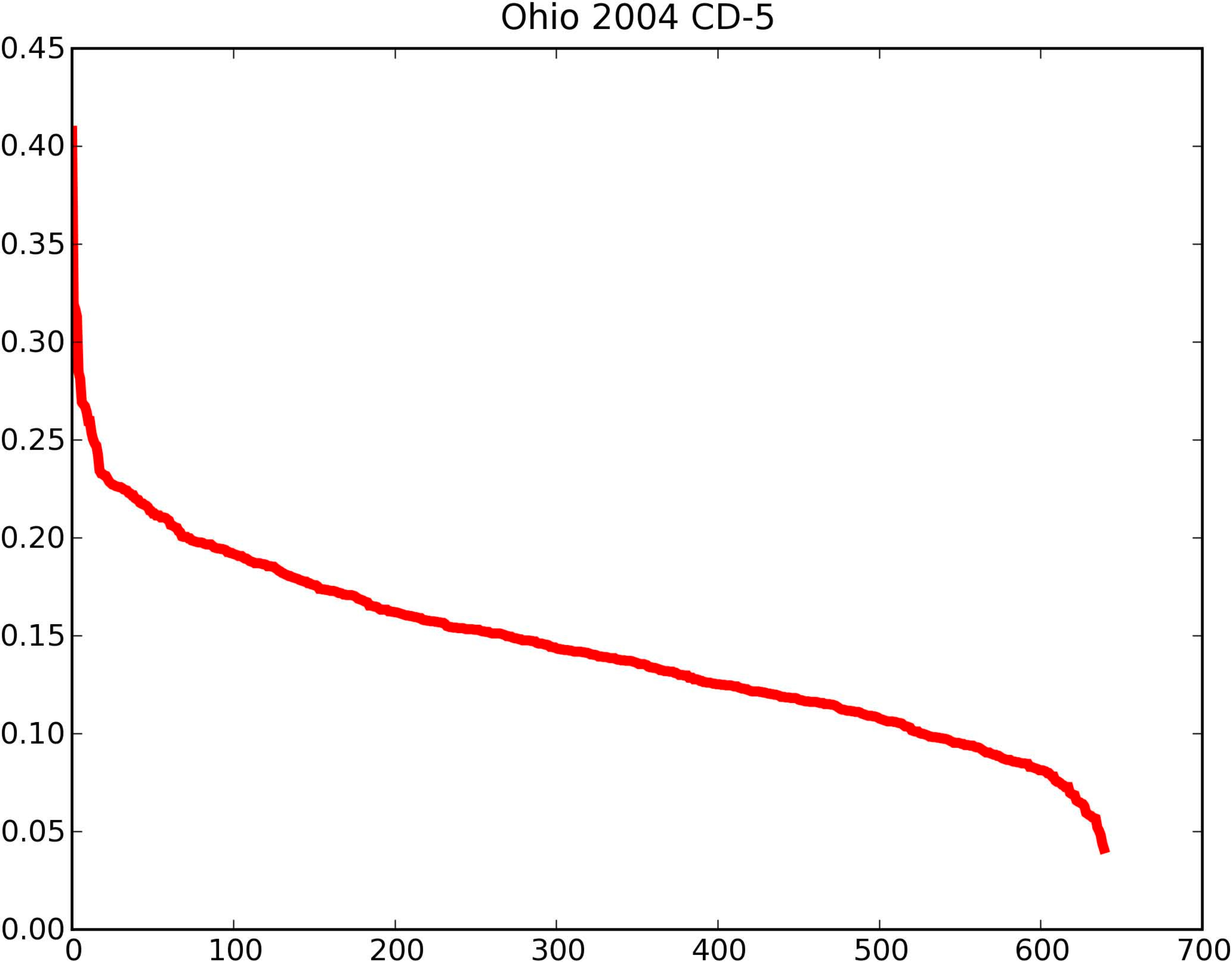
The ``negative-exponential'' auditing method (NEGEXP) is a heuristic basic auditing method. Intuitively, the probability that a precinct is audited is one minus a negative exponential function of the error bound for a precinct. See Figure 1.
The ``value'' to the adversary of corrupting precinct ![]() is assumed
to be
is assumed
to be ![]() , the known upper bound on the amount of error (in the
margin of victory) that can be introduced in precinct
, the known upper bound on the amount of error (in the
margin of victory) that can be introduced in precinct ![]() . In a
typical situation
. In a
typical situation ![]() might be proportional to
might be proportional to ![]() ; this is the
Linear Error Bound Assumption.
; this is the
Linear Error Bound Assumption.
Intuitively, the auditor wants to make the adversary's risk of detection grow with the ``value'' a precinct has to the adversary; this motivates the adversary to leave untouched those precincts with large error bounds. The adversary thus ends up having to corrupt a larger number of smaller precincts, which increases his or her chance of being caught in a random sample.
The motivation for the NEGEXP method is the following strategy for
the auditor: determine auditing probabilities so that
the chance of auditing at least one precinct from the set of corrupted precincts
depends only on the total error bound of that set of precincts.
For example, the adversary will then be
indifferent between corrupting a single precinct with error bound
![]() or corrupting two precincts with respective error bounds
or corrupting two precincts with respective error bounds
![]() and
and ![]() . The chance of being caught on
. The chance of being caught on
![]() or being caught on at least one of
or being caught on at least one of ![]() and
and ![]() should be the same.
should be the same.
This implies that the auditor does not audit
each ![]() with probability
with probability ![]() , where
, where
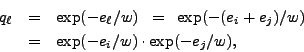
Our NEGEXP auditing method thus yields, from (5),
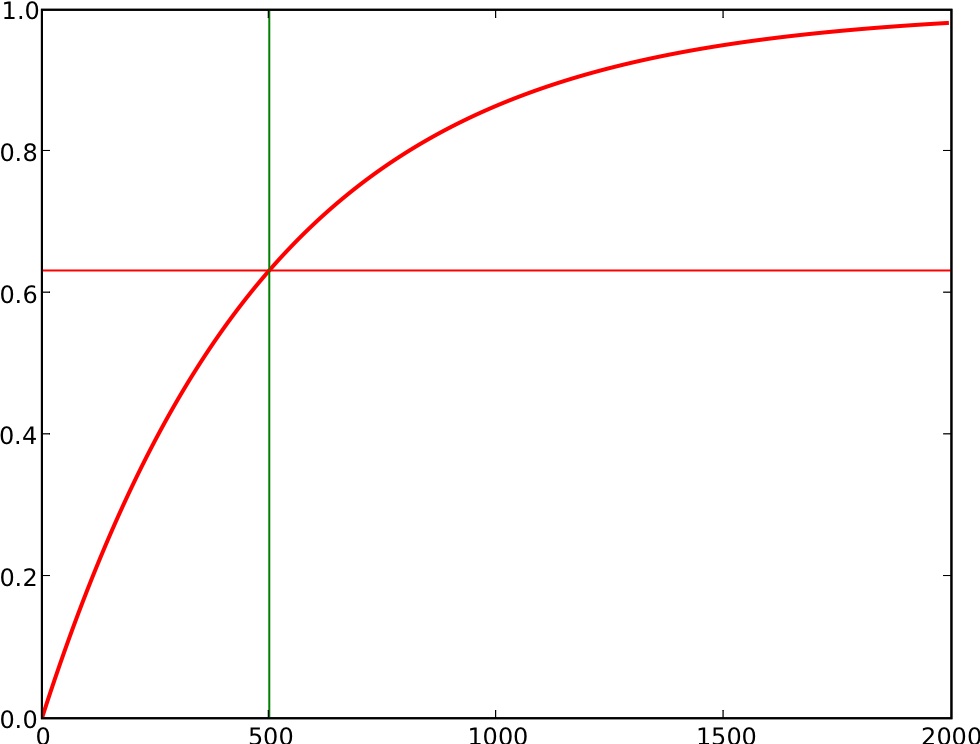
With the NEGEXP method, as the error bound ![]() increases, the probability of auditing
increases, the probability of auditing ![]() increases, starting off
at
increases, starting off
at ![]() for
for ![]() and increasing as
and increasing as ![]() increases, and levelling
off approaching
increases, and levelling
off approaching ![]() asymptotically for large
asymptotically for large ![]() . The chance of
auditing
. The chance of
auditing ![]() passes
passes
![]() as
as ![]() exceeds
exceeds ![]() .
.
|
The value ![]() can be thought of as approximating a ``threshold''
value: precincts with
can be thought of as approximating a ``threshold''
value: precincts with ![]() larger than
larger than ![]() have a fairly high probability of
being audited, while those smaller than
have a fairly high probability of
being audited, while those smaller than ![]() have a smaller chance of
being audited. As
have a smaller chance of
being audited. As ![]() decreases, the auditing gets more stringent:
more precincts are likely to be audited.
decreases, the auditing gets more stringent:
more precincts are likely to be audited.
An auditor may choose to use the NEGEXP auditing
method of equation (6), and choose ![]() to achieve an audit with a given significance level.
to achieve an audit with a given significance level.
The design of NEGEXP makes this easy, since
NEGEXP has the property
that for any set ![]() of precincts that the adversary may choose to
corrupt satisfying
of precincts that the adversary may choose to
corrupt satisfying
![]() the chance of detection is at least
the chance of detection is at least
This holds no matter what set of precincts, ![]() , the adversary chooses.
, the adversary chooses.
How can an auditor audit enough to achieve a given significance level? The relationship of equation (7)
gives a very nice way for the auditor
to choose ![]() : by choosing
: by choosing
| (9) |
| (10) |
This completes our description of the NEGEXP auditing method. Section 11 presents experimental results for this method. In the next section, we describe a different method (PPEBWR), which turns out to be nearly identical (but slightly better) in efficiency to the NEGEXP method, and which in some circumstances may be easier to work with, although it is somewhat less flexible.
This section presents the ``PPEBWR'' (sampling with probability proportional to error bound, with replacement) auditing strategy. It is simple to implement, and does at least as well as the NEGEXP method. Indeed, the PPEBWR is an excellent method in many respects, and we recommend its use, although the NEGEXP may be more useful when additional flexibility is required (e.g. having multiple races with overlapping jurisdictions).
Consider auditing an election with non-uniform error bounds
![]() where
where
![]() . Let
. Let ![]() be the
(minimum) level of error one wishes to detect;
be the
(minimum) level of error one wishes to detect; ![]() is the margin of
victory. Consider the following sampling-with-replacement procedure.
Form a sampling distribution
is the margin of
victory. Consider the following sampling-with-replacement procedure.
Form a sampling distribution ![]() over the precincts:
over the precincts:
While the per-round probabilities ![]() are
proportional to size, the overall probabilities
are
proportional to size, the overall probabilities ![]() are generally
not: note that as
are generally
not: note that as ![]() gets large the overall
probability of selection of each precinct approaches
gets large the overall
probability of selection of each precinct approaches ![]() . Actually,
the overall probabilities
. Actually,
the overall probabilities ![]() turn out to be nearly identical (but slightly
less) than those computed by the NEGEXP method.
turn out to be nearly identical (but slightly
less) than those computed by the NEGEXP method.
We now show how to determine the number ![]() of rounds for a desired
audit significance level
of rounds for a desired
audit significance level ![]() . Any set of precincts whose
total error bound is at least
. Any set of precincts whose
total error bound is at least ![]() will have probability weight at
least
will have probability weight at
least ![]() . Similar to the derivation in (12) where we replace
. Similar to the derivation in (12) where we replace ![]() by
by ![]() , the probability that at least one such precinct is detected is at least
, the probability that at least one such precinct is detected is at least
We can show that the probability ![]() with which any
given precinct
with which any
given precinct ![]() is audited is slightly smaller than the
negative-exponential audit probability leading to a slightly more efficient
sample size. Our experimental results have
shown that the difference in audit sizes of the two methods is nevertheless small.
is audited is slightly smaller than the
negative-exponential audit probability leading to a slightly more efficient
sample size. Our experimental results have
shown that the difference in audit sizes of the two methods is nevertheless small.
The costs of the PPEBWR strategy are easy to compute.
The expected number of precincts audited is
![]() and the expected number of votes audited is
and the expected number of votes audited is
![]()
Note that in both NEGEXP and PPEBWR the confidence level achieved is at least
![]() no matters what strategy the adversary follows (within the assumptions made). This includes the best possible strategy in which the adversary is aware of our auditing scheme and minimizes his detection probability; he/she still cannot lower this probability beyond
no matters what strategy the adversary follows (within the assumptions made). This includes the best possible strategy in which the adversary is aware of our auditing scheme and minimizes his detection probability; he/she still cannot lower this probability beyond ![]() .
.
This section drops the assumption that
error bounds are proportional to precinct size,
i.e., that
![]() How else can the auditor obtain a bound on the
error? Instead of having a size-dependent audit, he or she may
have a vote-dependent audit, using the fact that
How else can the auditor obtain a bound on the
error? Instead of having a size-dependent audit, he or she may
have a vote-dependent audit, using the fact that
![]() if
if
If we are unsure who the ``runner-up'' is,
we can take the maximum bound over any such ``runner-up'':
![]() Note that the ``candidates'' used for the ``invalid'' or ``undervote''
tallies should be excluded--they cannot be winners or runners-up.
These bounds
Note that the ``candidates'' used for the ``invalid'' or ``undervote''
tallies should be excluded--they cannot be winners or runners-up.
These bounds ![]() will usually be larger than those obtained via a
within-shift bound
will usually be larger than those obtained via a
within-shift bound ![]() , thus giving worse results.
However, in a two-candidate race if a precinct votes almost entirely
for the electronic runner-up, the new bound may be smaller.
, thus giving worse results.
However, in a two-candidate race if a precinct votes almost entirely
for the electronic runner-up, the new bound may be smaller.
Stark [19, Section 3.1] suggests ``pooling'' several obviously losing candidates to create an obviously losing ``pseudo-candidate'' to reduce the error bounds; this can also be applied here.
We illustrate and compare the previously described methods for handling variable-sized precincts using data from Ohio. These results show that taking precinct size into account (e.g. by using NEGEXP or PPSWR) can result in dramatic reductions in auditing cost, compared to methods (such as SAFE) that do not.
Mark Lindeman kindly supplied a dataset of precinct vote counts (sizes)
for the Ohio congressional district 5 race (OH-05) in 2004.
A total of ![]() votes were cast in 640 precincts, whose sizes ranged
from 1637 (largest) to 132 (smallest), a difference
by a factor of more than 12. See Figure 2.
votes were cast in 640 precincts, whose sizes ranged
from 1637 (largest) to 132 (smallest), a difference
by a factor of more than 12. See Figure 2.
|
Let us assume a margin of victory of ![]() :
:
![]() .
Assume the adversary changes at most
.
Assume the adversary changes at most ![]() of a precinct's votes,
and assume a confidence level of
of a precinct's votes,
and assume a confidence level of ![]() (
(![]() ).
).
If the precincts were equal-sized, the Rule of
Thumb [16] would suggest auditing ![]() precincts.
The more accurate APR formula (3) suggests auditing 93
precincts (here
precincts.
The more accurate APR formula (3) suggests auditing 93
precincts (here ![]() precincts). The expected workload would
be 45852 votes counted. But the precincts are quite far from being
equal-sized. If we sample 93 precincts uniformly (using the APR recommendation
inappropriately here, since the precincts are variable-sized), we now
only achieve a 67% confidence of detecting at least one corrupted
precinct, when the adversary has changed enough votes to change the
election outcome. The reason is that all of the corruption can fit in
the 7 largest precincts now.
precincts). The expected workload would
be 45852 votes counted. But the precincts are quite far from being
equal-sized. If we sample 93 precincts uniformly (using the APR recommendation
inappropriately here, since the precincts are variable-sized), we now
only achieve a 67% confidence of detecting at least one corrupted
precinct, when the adversary has changed enough votes to change the
election outcome. The reason is that all of the corruption can fit in
the 7 largest precincts now.
The SAFE auditing method [11]
would determine that ![]() (reduced from
(reduced from ![]() for the uniform case,
since now the adversary need only corrupt the 7 largest precincts to change
the election outcome). Using a uniform sampling procedure to have at least
a 92% chance of picking one of those 7 precincts (or any corrupted precinct)
requires a sample size of 193 precincts (chosen uniformly), and an expected
workload of 95,155 votes to recount.
for the uniform case,
since now the adversary need only corrupt the 7 largest precincts to change
the election outcome). Using a uniform sampling procedure to have at least
a 92% chance of picking one of those 7 precincts (or any corrupted precinct)
requires a sample size of 193 precincts (chosen uniformly), and an expected
workload of 95,155 votes to recount.
With the NEGEXP method, larger precincts are sampled
with greater probability. The adversary is thus prodded to disperse
his corruption more broadly, and thus needs to use more precincts,
which makes detecting the corruption easier for the auditor. The
NEGEXP method computes
![]() , and
audits a precinct of size
, and
audits a precinct of size ![]() with probability
with probability
![]() .
The largest precinct is audited with probability 0.408, while the
smallest is audited with probability 0.041.
The expected number of precincts selected for auditing is only 92.6, and
the expected workload is only 50,937 votes counted.
.
The largest precinct is audited with probability 0.408, while the
smallest is audited with probability 0.041.
The expected number of precincts selected for auditing is only 92.6, and
the expected workload is only 50,937 votes counted.
The PPEBWR method gave results almost identical to those for the NEGEXP method. The expected number of distinct precincts sampled was 91.6, and the expected workload was 50402 votes counted. Each precinct was sampled with a probability within 0.0031 of the corresponding probability for the NEGEXP method.
We see that for this example the NEGEXP method (or the PPEBWR method) is approximately twice as efficient (in terms of votes counted) as the SAFE method, for the same confidence level.
The program and datasets for our experiments are available at https://people.csail.mit.edu/rivest/pps/varsize.py, https://people.csail.mit.edu/rivest/pps/oh5votesonly.txt (Ohio).
The SAFE method may often be a poor choice when there are variable-precinct-sizes, particularly when there are a few very large precincts. One really needs a method that is tuned to variable-sized precincts by using variable auditing probabilities, rather than a method that uses uniform sampling probabilities.
The optimal auditing method can be represented as a
probability distribution assigning a probability ![]() to each
subset
to each
subset ![]() , where
, where ![]() indicates the probability that the
auditor will choose the subset of precincts,
indicates the probability that the
auditor will choose the subset of precincts, ![]() , for auditing. Since
there are
, for auditing. Since
there are ![]() such subsets, representing these probabilities
explicitly takes space exponential in
such subsets, representing these probabilities
explicitly takes space exponential in ![]() .
.
The optimal strategy can be found with linear programming, if the
number ![]() of precincts is not too large (say a dozen at most).
The linear programming formulation requires that
for each
subset
of precincts is not too large (say a dozen at most).
The linear programming formulation requires that
for each
subset ![]() of total error bound
of total error bound ![]() or more votes, the sum of the
probabilities of the subsets
or more votes, the sum of the
probabilities of the subsets ![]() having nonnegative intersection with
having nonnegative intersection with
![]() needs to be at least
needs to be at least ![]() .
.
![\begin{displaymath}
(\forall B)\left[
\left(\sum_{i\in B}e_i \ge M\right)
...
...t(\sum_{S:S\cap B \neq \phi}p_S \ge 1-\alpha\right)
\right]
\end{displaymath}](img168.png)
Finally, the objective function to be minimized is
the
expected number of votes to be recounted:
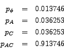
For example, suppose we have ![]() precincts
precincts ![]() with sizes
with sizes
![]() and error bounds
and error bounds
![]() ,
an adversarial corruption target
of
,
an adversarial corruption target
of ![]() votes, and a target significance level of
votes, and a target significance level of ![]() .
Then an optimal auditing strategy, when
the auditor is charged on a per-vote-recounted basis, is:
.
Then an optimal auditing strategy, when
the auditor is charged on a per-vote-recounted basis, is:
This approach is the ``gold standard'' for auditing with variable-sized precincts, in the sense that it definitely provides the most efficient procedure in terms of the stated optimization criterion. (We note that it is easy to refine this approach to handle the following variations: (1) an optimization criterion that is some linear combination of precincts counted and ballots counted and (2) a requirement that exactly (or at least, or at most) a certain number of precincts be audited.)
However, as noted, it may yield an auditing strategy with as many as
![]() potential actions (subsets to be audited) for the auditor, and so is not
efficient enough for real use, except for very small elections.
potential actions (subsets to be audited) for the auditor, and so is not
efficient enough for real use, except for very small elections.
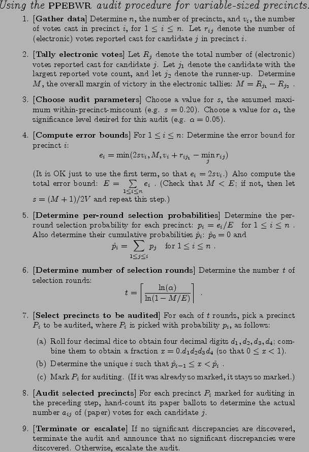
We recommend the use of the PPEBWR method for use in an audit in a simple election. It gives the most efficient audit, for a given confidence level, of the audit methods studied here (other than the optimal method, which is too inefficient for practical use). Figure 3 summarizes the PPEBWR audit procedure recommended for use.
In an election containing multiple races (possibly with overlapping jurisdictions), the NEGEXP method is the more flexible. See Section 13.2 for discussion.
If the error bounds are computed using only the Linear Error Bound Assumption,
so that ![]() , then the probability of picking precinct
, then the probability of picking precinct ![]() is just
is just
![]() , so that we are picking with ``probability proportional to size''--this
is then the PPSWR procedure.
When the Linear Error Bound Assumption is used, one is assuming that
errors larger than
, so that we are picking with ``probability proportional to size''--this
is then the PPSWR procedure.
When the Linear Error Bound Assumption is used, one is assuming that
errors larger than ![]() in a precinct will be noticed and caught
``by other means''; one should ensure that this indeed happens.
(Letting runners-up pick precincts to audit could be such a mechanism.)
in a precinct will be noticed and caught
``by other means''; one should ensure that this indeed happens.
(Letting runners-up pick precincts to audit could be such a mechanism.)
Other considerations may result in interesting and reasonable modifications. Letting runners-up pick precincts to audit is probably helpful, although these precincts should then be ignored during the PPEBWR portion of the audit.
The ``escalation'' procedure for enlarging the audit when significant
discrepancies are found is (intentionally) left rather unspecified
here. We recommend reading Stark [19] for guidance. At one
extreme, one can perform a full recount of all votes cast. More
reasonably, one can utilize a staged procedure, where the error budget
![]() is allocated among the stages; only if enough new
discrepancies are discovered in one stage does auditing proceed to the
next.
is allocated among the stages; only if enough new
discrepancies are discovered in one stage does auditing proceed to the
next.
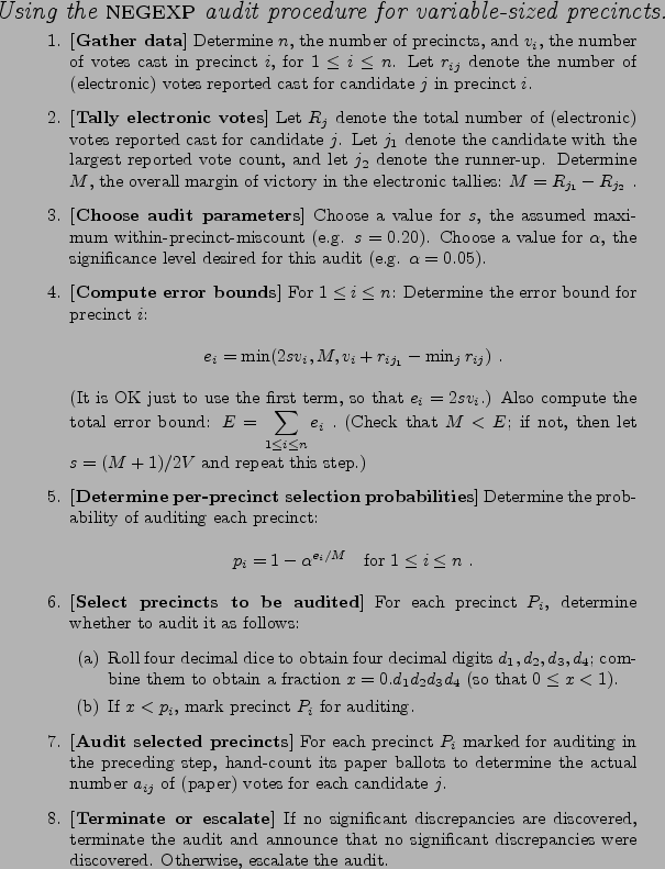
Figure 4 summarizes the NEGEXP audit procedure recommended for use. The NEGEXP method seems intrinsically more flexible than the PPEBWR method.
NEGEXP can handle multiple races with overlapping jurisdictions such that each precinct is audited at most once even when it is marked for auditing in multiple races. As with any basic auditing method, each precinct is audited independently with a precinct-specific probability. Assume that when a precinct is audited, we audit all races voted on in that precinct. Since the results for each race may imply a different auditing probability for the precinct, it suffices to audit the precinct with the maximum of the probabilities corresponding to the different races.
In a similar manner, the NEGEXP method can be used when the
auditing probabilities need to be changed (e.g. because of the effect
of late-reporting jurisdictions). Assume that the auditing probability
changes from ![]() to
to ![]() . If the precinct was audited in the first audit, nothing additional needs to be done.
If the precinct was not audited and
. If the precinct was audited in the first audit, nothing additional needs to be done.
If the precinct was not audited and ![]() , nothing needs to be done because we already audited the precinct
with a larger probability than we need to. Otherwise (when
, nothing needs to be done because we already audited the precinct
with a larger probability than we need to. Otherwise (when ![]() ), a dice-roll with probability
), a dice-roll with probability ![]() should be used to determine if the precinct should now be audited. The additional dice-roll ensures that the overall probability of auditing the precinct in discussion is
should be used to determine if the precinct should now be audited. The additional dice-roll ensures that the overall probability of auditing the precinct in discussion is ![]() , the final auditing probability.
, the final auditing probability.
It would be preferable in general, rather than having to deal with precincts of widely differing sizes, if one could somehow group the records for the larger precincts into ``bins'' for ``pseudo-precincts'' of some smaller standard size. (One can do this for say paper absentee ballots, by dividing the paper ballots into nominal standard precinct-sized batches before scanning them.) It is harder to do this if you have DRE's with wide disparities between the number of voters voting on each such machine. See Neff [12] and Wand [22] for further discussion.
We have presented two useful post-election auditing procedures: a powerful and flexible ``negative-exponential'' (NEGEXP) method, and a slightly more efficient ``sampling with probability proportional to size, with replacement'' (PPEBWR) method.
Thanks to Mark Lindeman for helpful discussions and the Ohio dataset. Thanks also to Kathy Dopp, Andy Drucker, Silvio Micali, Howard Stanislevic, Christos Papadimitriou, and Jerry Lobdill for constructive suggestions. Thanks to Phil Stark for his detailed feedback and pointers to the financial auditing literature.
This document was generated using the LaTeX2HTML translator Version 2002-2-1 (1.71)
Copyright © 1993, 1994, 1995, 1996,
Nikos Drakos,
Computer Based Learning Unit, University of Leeds.
Copyright © 1997, 1998, 1999,
Ross Moore,
Mathematics Department, Macquarie University, Sydney.
The command line arguments were:
latex2html -split 0 -show_section_numbers -local_icons -no_navigation varsize.tex
The translation was initiated by Raluca Ada Popa on 2008-06-30