Experimental evidence alone is insufficient to allow us to make strong statements about Nice's non-interference properties for general network topologies, background flow workloads, and foreground flow workloads. We therefore analyze it formally to bound the reduction in throughput that Nice imposes on foreground flows. Our primary result is that under a simplified network model, for long transfers, the reduction in the throughput of Reno flows is asymptotically bounded by a factor that falls exponentially with the maximum queue length of the bottleneck router irrespective of the number of Nice flows present.
Theoretical analysis of network protocols, of course, has limits. In general, as one abstracts away details to gain tractability or generality, one risks omitting important behaviors. Most significantly, our formal analysis assumes a simplified fluid approximation and synchronous network model, as described below. Also, our formal analysis holds for long background flows, which are the target workload of our abstraction. But it also assumes long foreground Reno flows, which are clearly not the only cross-traffic of interest. Finally, in our analysis, we abstract detection by assuming that at the end of each RTT epoch, a Nice sender accurately estimates the queue length during the previous epoch. Although these assumptions are restrictive, the insights gained in the analysis lead us to expect the protocol to work well under more general circumstances. The analysis has also guided our design, allowing us to include features that are necessary for noninterference while excluding those that are not. Our experience with the prototype has supported the benefit of using theoretical analysis to guide our design: we encountered few surprises and required no topology or workload-dependent tuning during our experimental effort.
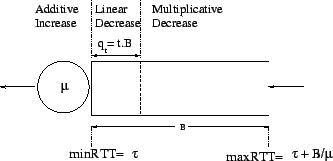
We use a simplified fluid approximation model of the network
to help us model the interaction of multiple flows
using separate congestion control algorithms.
This model assumes infinitely small packets. We simplify the network
itself to a source,
destination, and a single bottleneck, namely a router that performs drop-tail queuing as
shown in Figure 1.
Let ![]() denote the service rate of the queue and
denote the service rate of the queue and ![]() the buffer capacity at the queue.
Let
the buffer capacity at the queue.
Let ![]() be the round-trip delay of packets between the source and
destination excluding all queuing delays. We consider a fixed number
of connections,
be the round-trip delay of packets between the source and
destination excluding all queuing delays. We consider a fixed number
of connections, ![]() following
Reno and
following
Reno and ![]() following Nice, each of which has one continuously
backlogged flow between a source and a destination.
Let
following Nice, each of which has one continuously
backlogged flow between a source and a destination.
Let
![]() be the Nice threshold and
be the Nice threshold and ![]() be the corresponding queue
size that triggers multiplicative backoff for Nice flows. The
connections are homogeneous, i.e. they experience the same
propagation delay
be the corresponding queue
size that triggers multiplicative backoff for Nice flows. The
connections are homogeneous, i.e. they experience the same
propagation delay ![]() . Moreover, the connections are
synchronized so that
in the case of buffer overflow, all connections simultaneously
detect a loss and multiply their window sizes by
. Moreover, the connections are
synchronized so that
in the case of buffer overflow, all connections simultaneously
detect a loss and multiply their window sizes by ![]() .
Models assuming flow synchronization have been used in previous
analyses [6]. We model only the congestion avoidance phase to
analyze the steady-state behavior.
.
Models assuming flow synchronization have been used in previous
analyses [6]. We model only the congestion avoidance phase to
analyze the steady-state behavior.
We obtain a bound on the reduction in the throughput of Reno flows due to the presence of Nice flows by analyzing the dynamics of the bottleneck queue. We achieve this goal by dividing the duration of the flows into periods. In each period we bound the decrease in the number of Reno packets processed by the router due to interfering Nice packets. In the following we give an outline of this analysis. The complete analysis with detailed proofs appears in the our technical report [49].
Let ![]() and
and ![]() denote respectively the total number of
outstanding Reno and Nice packets in the network at time
denote respectively the total number of
outstanding Reno and Nice packets in the network at time ![]() .
.
![]() , the total window size, is
, the total window size, is
![]() . We trace
these window sizes across periods.
The end of a period and the beginning of the next
is marked by a packet loss, at which time each flow reduces its window
size by a factor of
. We trace
these window sizes across periods.
The end of a period and the beginning of the next
is marked by a packet loss, at which time each flow reduces its window
size by a factor of ![]() .
.
![]() just
before a loss and
just
before a loss and
![]() just after. Let
just after. Let
![]() be the
beginning of one such period after a loss.
Consider the
case when
be the
beginning of one such period after a loss.
Consider the
case when
![]() and
and ![]() . For ease of
analysis we assume that the ``Vegas
. For ease of
analysis we assume that the ``Vegas ![]() '' parameter for the Nice
flows is
'' parameter for the Nice
flows is ![]() , i.e. the Nice flows additively decrease upon
observing round-trip times greater than
, i.e. the Nice flows additively decrease upon
observing round-trip times greater than ![]() .
The window dynamics in any period can be split into
three intervals as described below.
.
The window dynamics in any period can be split into
three intervals as described below.
Additive Increase, Additive Increase: In this interval ![]() both Reno and
Nice flows increase linearly.
both Reno and
Nice flows increase linearly.
![]() increases from
increases from ![]() to
to
![]() , at which point the queue
starts building.
, at which point the queue
starts building.
Additive Increase, Additive Decrease: This interval
![]() is marked by additive increase of
is marked by additive increase of ![]() ,
but additive decrease of
,
but additive decrease of ![]() as the ``
as the ``
![]() " rule
triggers the underlying Vegas controls for the Nice flows.
The end of this interval is marked by
" rule
triggers the underlying Vegas controls for the Nice flows.
The end of this interval is marked by
![]() .
.
Additive Increase, Multiplicative Decrease: In this interval
![]() ,
, ![]() multiplicatively decreases in response to
observing queue lengths above
multiplicatively decreases in response to
observing queue lengths above ![]() .
However, the rate of decrease
of
.
However, the rate of decrease
of ![]() is bounded by the rate of increase of
is bounded by the rate of increase of
![]() , as any faster a decrease will cause the queue size to drop
below
, as any faster a decrease will cause the queue size to drop
below ![]() .
At the end of this interval
.
At the end of this interval
![]() . At this point, each flow
decreases its window size by a factor of
. At this point, each flow
decreases its window size by a factor of ![]() , thereby entering into
the next period.
, thereby entering into
the next period.
In order to quantify the interference experienced by Reno flows
because of the presence of Nice flows, we formulate differential
equations to represent the variation of the queue size in a period. We
then show that the values of ![]() and
and ![]() at the beginning of
periods stabilize after several losses, so that the length of a period
converges to a fixed value. It is then straightforward to compute the
total amount of Reno flow sent out in a period.
We show in the technical report [49] that the interference
at the beginning of
periods stabilize after several losses, so that the length of a period
converges to a fixed value. It is then straightforward to compute the
total amount of Reno flow sent out in a period.
We show in the technical report [49] that the interference ![]() ,
defined as the
fractional loss in throughput experienced by Reno flows because of
the presence of Nice flows, is given as follows.
,
defined as the
fractional loss in throughput experienced by Reno flows because of
the presence of Nice flows, is given as follows.
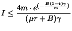
Theorem 1: The interference ![]() is given by
is given by