|
USENIX 2002 Annual Technical Conference Paper
[USENIX 2002 Technical Program Index]
| Pp. 317-327 of the Proceedings |  |
Robust Positioning Algorithms for Distributed Ad-Hoc Wireless Sensor Networks
Chris Savarese
Jan Rabaey
Berkeley Wireless Research Center
{savarese,jan}@eecs.berkeley.edu
Koen Langendoen
Faculty of Information Technology and Systems
Delft University of Technology, The Netherlands
koen@pds.twi.tudelft.nl
A distributed algorithm for determining the positions of nodes in
an ad-hoc, wireless sensor network is explained in detail. Details
regarding the implementation of such an algorithm are also discussed.
Experimentation is performed on networks containing 400 nodes randomly
placed within a square area, and resulting error magnitudes are
represented as percentages of each node's radio range. In scenarios
with 5% errors in distance measurements, 5% anchor node population
(nodes with known locations), and average connectivity levels between
neighbors of 7 nodes, the algorithm is shown to have errors less than
33% on average. It is also shown that, given an average connectivity
of at least 12 nodes and 10% anchors, the algorithm performs well with
up to 40% errors in distance measurements.
Ad-hoc wireless sensor networks are being developed for use in monitoring
a host of environmental characteristics across the area of deployment,
such as light, temperature, sound, and many others. Most of these data
have the common characteristic that they are useful only when considered
in the context of where the data were measured, and so most sensor data
will be stamped with position information. As these are ad-hoc networks,
however, acquiring this position data can be quite challenging.
Ad-hoc systems strive to incorporate as few assumptions as possible about
characteristics such as the composition of the network, the relative
positioning of nodes, and the environment in which the network operates.
This calls for robust algorithms that are capable of handling the
wide set of possible scenarios left open by so many degrees of freedom.
Specifically, we only assume that all the nodes being considered in
an instance of the positioning problem are within the same connected
network, and that there will exist within this network a minimum of
four anchor nodes. Here, a connected network is a network in which
there is a path between every pair of nodes, and an anchor
node is a node that is given a priori knowledge of its position with
respect to some global coordinate system.
A consequence of the ad-hoc nature of these networks is the lack
of infrastructure inherent to them. With very few exceptions, all
nodes are considered equal; this makes it difficult to rely on centralized
computation to solve network wide problems, such as positioning. Thus, we
consider distributed algorithms that achieve robustness through iterative
propagation of information through a network.
The positioning algorithm being considered relies on measurements, with
limited accuracy, of the distances between pairs of neighboring nodes;
we call these range measurements. Several techniques can be used to
generate these range measurements, including time of arrival, angle of
arrival, phase measurements, and received signal strength. This algorithm
is indifferent to which method is used, except that different methods
offer different tradeoffs between accuracy, complexity, cost, and
power requirements. Some of these methods generate range measurements
with errors as large as  50% of the measurement. Note that these
errors can come from multiple sources, including multipath interference,
line-of-sight obstruction, and channel inhomogeneity with regard to
direction. This work, however, is not concerned with the problem of
determining accurate range measurements. Instead, we assume large errors
in range measurements that should represent an agglomeration of multiple
sources of error. Being able to cope with range measurements errors is
the first of two major challenges in positioning within an ad-hoc space,
and will be termed the range error problem throughout this paper. 50% of the measurement. Note that these
errors can come from multiple sources, including multipath interference,
line-of-sight obstruction, and channel inhomogeneity with regard to
direction. This work, however, is not concerned with the problem of
determining accurate range measurements. Instead, we assume large errors
in range measurements that should represent an agglomeration of multiple
sources of error. Being able to cope with range measurements errors is
the first of two major challenges in positioning within an ad-hoc space,
and will be termed the range error problem throughout this paper.
The second major challenge behind ad-hoc positioning algorithms,
henceforth referred to as the sparse anchor node problem, comes
from the need for at least four reference points with known location in
a three-dimensional space in order to uniquely determine the location of
an unknown object. Too few reference points results in ambiguities that
lead to underdetermined systems of equations. Recalling the assumptions
made above, only the anchor nodes will have positioning information at the
start of these algorithms, and we assume that these anchor nodes will be
located randomly throughout an arbitrarily large network. Given limited
radio ranges, it is therefore highly unlikely that any randomly selected
node in the network will be in direct communication with a sufficient
number of reference points to derive its own position estimate.
In response to these two primary obstacles, we present an algorithm
split into two phases: the start-up phase and the refinement
phase. The start-up phase addresses the sparse anchor node problem
by cooperatively spreading awareness of the anchor nodes' positions
throughout the network, allowing all nodes to arrive at initial position
estimates. These initial estimates are not expected to be very accurate,
but are useful as rough approximations. The refinement phase of the
algorithm then uses the results of the start-up algorithm to improve
upon these initial position estimates. It is here that the range error
problem is addressed.
This paper presents our algorithms in detail, and discusses several
network design guidelines that should be taken into consideration when
deploying a system with such an algorithm. Section 2
will discuss related work in this field. Section 3 will
elaborate our two-phase algorithm approach, exploring in depth the
start-up and refinement phases of our solution. Section 4
will discuss some subtleties of the algorithm in relation to our
simulation environment. Section 5 reports on the experiments
performed to characterize the performance of our algorithm. Finally,
Section 6 is a discussion of design guidelines and algorithm
limitations, and Section 7 concludes the paper.
Related work
The recent survey and taxonomy by Hightower and Borriello
provides a general overview of the state of the art in location
systems [7]. However, few systems for locating sensor
nodes in an ad-hoc network are described, because of the aforementioned
range error and sparse anchor node problems. Many systems are based
on the attractive option of using the RF radio for measuring the range
between nodes, for example, by observing the signal strength. Experience
has shown, however, that this approach yields very inaccurate
distances [8]. Much better results are obtained by
time-of-flight measurements, particularly when acoustic and RF signals are
combined [6,12]; accuracies of a few percent
of the transmission range are reported. Acoustic signals, however,
are temperature dependent and require an unobstructed line of sight.
Furthermore, even small errors do accumulate when propagating distance
information over multiple hops.
A drastic approach that avoids the range error problem altogether is
to use only connectivity between nodes. The GPS-less system by Bulusu
et al. [3] employs a grid of beacon nodes with known
locations; each unknown node sets its position to the centroid of the
locations of the beacons connected to the unknown. The position
accuracy is about one-third of the separation distance between beacons,
implying a high beacon density for practical purposes. Doherty et al. use
the connectivity between nodes to formulate a set of geometric constraints
and solve it using convex optimization [5]. The
resulting accuracy depends on the fraction of anchor nodes. For example,
with 10% anchors the accuracy for unknowns is on the order of the
radio range. A serious drawback, which is currently being addressed,
is that convex optimization is performed by a single, centralized
node. The ``DV-hop'' approach by Niculescu and Nath, in contrast, is
completely ad-hoc and achieves an accuracy of about one-third of the
radio range for networks with dense populations of (highly connected)
nodes [10]. In a first phase anchors flood their location
to all nodes in the network. Each unknown node records the position and
(minimum) number of hops to at least three anchors. Whenever an anchor
 infers the position of another anchor infers the position of another anchor  it computes the distance
between them, divides that by the number of hops, and floods this average
hop distance into the network. Each unknown uses the average hop distance
to convert hop counts to distances, and then performs a triangulation to
three or more distant anchors to estimate its own position. ``DV-hop''
works well in dense and regular topologies, but for sparse or irregular
networks the accuracy degrades to the radio range. it computes the distance
between them, divides that by the number of hops, and floods this average
hop distance into the network. Each unknown uses the average hop distance
to convert hop counts to distances, and then performs a triangulation to
three or more distant anchors to estimate its own position. ``DV-hop''
works well in dense and regular topologies, but for sparse or irregular
networks the accuracy degrades to the radio range.
More accurate positions can be obtained by using the range measurements
between individual nodes (when the errors are small). When the
fraction of anchor nodes is high the ``iterative multilateration''
method by Savvides et al. can be used [12]. Nodes
that are connected to at least three anchors compute their
position and upgrade to anchor status, allowing additional
unknowns to compute their position in the next iteration, etc.
Recently a number of approaches have been proposed that require few
anchors [4,9,10,11]. They
are quite similar and operate as follows. A node measures the distances
to its neighbors and then broadcasts this information. This results
in each node knowing the distance to its neighbors and some
distances between those neighbors. This allows for the construction of
(partial) local maps with relative positions. Adjacent local maps are
combined by aligning (mirroring, rotating) the coordinate systems. The
known positions of the anchor nodes are used to obtain maps with absolute
positions. When three or more anchors are present in the network a single
absolute map results. This style of locationing is not very robust since
range errors accumulate when combining the maps.
Two-phase positioning
As mentioned earlier, the two primary obstacles to positioning in an
ad-hoc network are the sparse anchor node problem and the range error
problem. In order to address each of these problems sufficiently,
our algorithm is separated into two phases: start-up and refinement.
For the start-up phase we use Hop-TERRAIN, an in-house algorithm
similar to DV-hop [10]. The Hop-TERRAIN algorithm
is run once at the beginning of the positioning algorithm to
overcome the sparse anchor node problem, and the Refinement algorithm
is run iteratively afterwards to improve upon and refine the position
estimates generated by Hop-TERRAIN. Note therefore that the emphasis
for Hop-TERRAIN is not on getting highly accurate position estimates,
but instead on getting very rough estimates so as to have a starting
point for Refinement. Conversely, Refinement is concerned only with nodes
that exist within a one-hop neighborhood, and it focuses on increasing
the accuracy of the position estimates as much as possible.
Hop-TERRAIN
Before the positioning algorithm has started, most of the nodes in a
network have no positioning data, with the exception of the anchors.
The networks being considered for this algorithm will be scalable to
very large numbers of nodes spread over large areas,
relative to the short radio ranges that each of the nodes is expected
to possess. Furthermore, it is expected that the percentage of nodes
that are anchor nodes will be small. This results in a situation in
which only a very small percentage of the nodes in the network are able
to establish direct contact with any of the anchors, and probably none
of the nodes in the network will be able to directly contact enough
anchors to derive a position estimate.
In order to overcome this initial information deficiency, the Hop-TERRAIN
algorithm finds the number of hops from a node to each of the anchors
nodes in a network and then multiplies this hop count by an
average hop distance (see Section 4.2) to estimate the range between the node and each
anchor. These computed ranges are then used together with the anchor
nodes' known positions to perform a triangulation and get the node's
estimated position. The triangulation consists of solving a system of
linearized equations (Ax=b) by means of a least squares algorithm,
as in earlier work [11].
Each of the anchor nodes launches the Hop-TERRAIN algorithm by initiating
a broadcast containing its known location and a hop count of 0. All of
the one-hop neighbors surrounding an anchor hear this broadcast, record
the anchor's position and a hop count of 1, and then perform another
broadcast containing the anchor's position and a hop count of 1.
Every node that hears this broadcast and did not hear the previous
broadcasts will record the anchor's position and a hop count of 2 and
then rebroadcast. This process continues until each anchor's position
and an associated hop count value have been spread to every node in
the network. It is important that nodes receiving these broadcasts
search for the smallest number of hops to each anchor.
This ensures conformity with the model used to estimate the average
distance of a hop, and it also greatly reduces network traffic.
As broadcasts may be omni-directional, and may therefore reach nodes
behind the broadcasting node (relative to the direction of the flow of
information), this algorithm causes nodes to hear many more packets than
necessary. In order to prevent an infinite loop of broadcasts, nodes
are allowed to broadcast information only if it is not stale to them.
In this context, information is stale if it refers to an anchor that the
node has already heard from and if the hop count included in the arriving
packet is greater than or equal to the hop count stored in memory for
this particular anchor. New information will always trigger a broadcast,
whereas stale information will never trigger a broadcast.
Once a node has received an average hop distance and data regarding at
least 3(4) anchor nodes for a network existing in a 2(3)-dimensional
space, it is able to perform a triangulation to estimate its location.
If this node subsequently receives new data after already having
performed a triangulation, either a smaller hop count or a new anchor,
the node simply performs another triangulation to include the new data.
This procedure is summarized in the following piece of pseudo code:
when a positioning packet is received,
if new anchor or lower hop count
then
store hop count for this anchor.
broadcast new packet for this anchor with
hop count = (hop count + 1).
else
do nothing.
if average hop count is known and
number of anchors  (dimension of space + 1) (dimension of space + 1)
then
triangulate.
else
do nothing.
The resulting position estimate is likely to be coarse in terms of
accuracy, but it provides an initial condition from which Refinement
can launch. The performance of this algorithm is discussed in detail
in Section 5.
Given the initial position estimates of Hop-TERRAIN in the start-up
phase, the objective of the refinement phase is to obtain more accurate
positions using the estimated ranges between nodes. Since Refinement must
operate in an ad-hoc network, only the distances to the direct (one-hop)
neighbors of a node are considered. This limitation allows Refinement to
scale to arbitrary network sizes and to operate on low-level networks that
do not support multi-hop routing (only a local broadcast is required).
Refinement is an iterative algorithm in which the nodes update their
positions in a number of steps. At the beginning of each step a node
broadcasts its position estimate, receives the positions and corresponding
range estimates from its neighbors, and computes a least squares
triangulation solution to determine its new position. In many cases
the constraints imposed by the distances to the neighboring locations
will force the new position towards the true position of the node. When,
after a number of iterations, the position update becomes small Refinement
stops and reports the final position. Note that Refinement is by nature
an ad-hoc (distributed) algorithm.
The beauty of Refinement is its simplicity, but that also limits its
applicability. In particular, it was a priori not clear under what
conditions Refinement would converge and how accurate the final solution
would be. A number of factors that influence the convergence and accuracy
of iterative Refinement are:

- the accuracy of the initial position estimates,
-
- the magnitude of errors in the range estimates,
-
- the average number of neighbors, and
-
- the fraction of anchor nodes.
Based on previous experience we assume that redundancy can counter the
above influences to a large extent. When a node has more than 3(4)
neighbors in a 2(3)-dimensional space the induced system of linear
equations is over-defined and errors will be averaged out by the least
squares solver. For example, data collected by Beutel [1]
shows that large range errors (standard deviation of 50%) can be
tolerated when locating a node surrounded by 5 (or more) anchors in a
2-dimensional space: the average distance between the estimated and true
position of the node is less than 5% of the radio range.
Despite the positive effects from redundancy we observed that a
straightforward application of Refinement did not converge in a
considerable number of ``reasonable'' cases. Close inspection of the
sequence of steps taken under Refinement revealed two important causes:
- 1.
- Errors propagate fast throughout the whole network. If the
network has a diameter
 , then an error introduced by a node
in step , then an error introduced by a node
in step  has (indirectly) affected every node in the network by step has (indirectly) affected every node in the network by step
 because of the triangulate-hop-triangulate-hop because of the triangulate-hop-triangulate-hop pattern. pattern.
- 2.
- Some network topologies are inherently hard, or even impossible,
to locate. For example, a cluster of
 nodes (no anchors) connected
by a single link to the main network can be simply rotated around the
`entry'-point into the network while keeping the exact same intra-
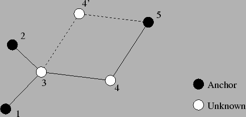
node ranges. Another example is given in Figure 1. nodes (no anchors) connected
by a single link to the main network can be simply rotated around the
`entry'-point into the network while keeping the exact same intra-
node ranges. Another example is given in Figure 1.
To mitigate error propagation we modified the refinement algorithm to
include a confidence associated with each node's position. The confidences
are used to weigh the equations when solving the system of linear
equations. Instead of solving Ax=b we now solve  Ax=b,
where is the vector of confidence weights. Nodes, like anchors, that
have high faith in their position estimates select high confidence values
(close to 1). A node that observes poor conditions (e.g., few neighbors,
poor constellation) associates a low confidence (close to 0) with its
position estimate, and consequently has less impact on the outcome of
the triangulations performed by its neighbors. The details of confidence
selection will be discussed in Section 4.3. The usage of
confidence weights improved the behavior of Refinement greatly: almost all
cases converge now, and the accuracy of the positions is also improved
considerably. Ax=b,
where is the vector of confidence weights. Nodes, like anchors, that
have high faith in their position estimates select high confidence values
(close to 1). A node that observes poor conditions (e.g., few neighbors,
poor constellation) associates a low confidence (close to 0) with its
position estimate, and consequently has less impact on the outcome of
the triangulations performed by its neighbors. The details of confidence
selection will be discussed in Section 4.3. The usage of
confidence weights improved the behavior of Refinement greatly: almost all
cases converge now, and the accuracy of the positions is also improved
considerably.
Another improvement to Refinement was necessary to handle the second
issue of ill-connected groups of nodes. Detecting that a single node is
ill-connected is easy: if the number of neighbors is less than 3(4) then
the node is ill-connected in a 2(3)-dimensional space. Detecting that
a group of nodes is ill-connected, however, is more complicated since
some global overview is necessary. We employ a heuristic that operates
in an ad-hoc fashion (no centralized computation), yet is able to detect
most ill-connected nodes. The underlying premise for the heuristic is
that a sound node has independent references to at least 3(4)
anchors. That is, the multi-hop routes to the anchors have no link
(edge) in common. For example, node 3 in Figure 1 (which is taken
from [12]) meets this criteria and is considered sound.
Figure 1:
Example topology.
 |
To determine if a node is sound, the Hop-TERRAIN algorithm records
the ID of each node's immediate neighbor along a shortest path to
each anchor. When multiple shortest paths are available, the first one
discovered is used (this only approximates the intended condition but
is considerably simpler). These IDs are collected in a set of sound
neighbors. When the number of unique IDs in this set reaches 3(4), a node
declares itself sound and may enter the Refinement phase. The neighbors
of the sound node add its ID to their sets and may in turn become sound
if their sound sets become sufficient. This process continues throughout
the network. The end result is that most ill-connected nodes will not
be able to fill their sets of sound neighbors with enough entries and,
therefore, may not participate in the Refinement phase. In the example
topology in Figure 1, node 3 will become sound, but node 4
will not. We also note that the more restrictive participating
node definition by Savvides et al. renders both unknown nodes as
ill-conditioned [12].
Refinement with both modifications (confidence weights, detection of
ill-connected nodes) performs quite satisfactorily, as will be shown by
the experiments in Section 5.
Simulation and algorithm details
To study the robustness of our two-phase positioning algorithm we created
a simulation environment in which we can easily control a number of
(network) parameters. We implemented the Hop-TERRAIN and Refinement
algorithms as C++ code running under the control of the OMNeT++ discrete
event simulator [13]. The algorithms are event driven, where
an event can be an incoming message or a periodic timer. Processing an
event usually involves updating internal state, and often generates
output messages that must be broadcast. All simulated sensor nodes
run exactly the same C++ code. The OMNeT++ library is in control of
the simulated time and enforces a semi-concurrent execution of the code
`running' on the multiple sensor nodes.
Although our positioning algorithm is designed to be used in an ad-hoc
network that presumably employs multi-hop routing algorithms, our
algorithm only requires that a node be able to broadcast a message
to all of its one hop neighbors. An important result of this is the
ability for system designers to allow the routing protocols to rely on
position information, rather than the positioning algorithm relying on
routing capabilities.
An important issue is whether or not the network provides reliable
communication in the presence of concurrent transmission. In this
paper we assume that message loss or corruption does not occur and that
each message is delivered at the neighbors within a fixed radio range
( ) from the sending node. Concurrent transmissions are allowed when
the transmission areas (circles) do not overlap. A node wanting to
broadcast a message while another message in its area is in progress
must wait until that transmission (and possibly other queued messages)
completes. In effect we employ a CSMA policy. ) from the sending node. Concurrent transmissions are allowed when
the transmission areas (circles) do not overlap. A node wanting to
broadcast a message while another message in its area is in progress
must wait until that transmission (and possibly other queued messages)
completes. In effect we employ a CSMA policy.
The functionality of the network layer (local broadcast) is implemented in
a single OMNeT++ object, which is connected to all sensor-node objects in
the simulation. This network object holds the topology of the simulated
sensor network, which can be read from a "scenario" file or generated
at random at initialization time. At time zero the network object sends
a pseudo message to each sensor-node object telling its role (anchor
or unknown) and some attributes (e.g., the position in the case of an anchor
node). From then on it relays messages generated by sensor nodes to the
sender's neighbors within a radius of units.
Hop-TERRAIN
At time zero of the Hop-TERRAIN algorithm, all of the nodes in the
network are waiting to receive hop count packets informing them of the
positions and hop distances associated with each of the anchor nodes.
Also at time zero, each of the anchor nodes in the network broadcasts a
hop count packet, which is received and repeated by all of the anchors'
one-hop neighbors. This information is propagated throughout the network
until, ideally, all the nodes in the network have positions and hop counts
for all of the anchors in the network as well as an average hop distance
(see below). At this point, each of the nodes performs a triangulation
to create an initial estimate of its position. The number of anchors
in any particular scenario is not known by the nodes in the network,
however, so it is difficult to define a stopping criteria to dictate
when a node should stop waiting for more information before performing a
triangulation. To solve this problem, nodes perform triangulations every
time they receive information that is not stale after having received
information from the first 3(4) anchors in a 2(3)-dimensional space (see
Section 3.1 for a definition of stale information).
Nodes also rely on the anchor nodes to inform them of the value to use for
the assumed average hop distance used in calculating the estimated range
to each anchor. Initially we experimented with simply using the maximum
radio range for this quantity. Better position results, however, are
attained by dynamically determining the average hop distance by comparing
the number of hops between the anchors themselves to the known distances
separating them following the calibration procedure used for DV-hop (see
Section 2). We implemented the calibration procedure
as a separate pass that follows the initial hop-count flooding. When
an anchor node receives a hop count from another anchor it computes
its estimate of the average hop distance, and floods that back into
the network. Nodes wait for the first such estimate to arrive before
performing any triangulation as outlined above. Subsequent estimates
from other anchor pairs are simply discarded to reduce network load.
The above details are sufficient for controlling the Hop-TERRAIN algorithm
within a simulated environment where all of the nodes start up at the same
time. One important consequence of a real network, however, is that the
nodes in the network start up or enter the network at random times,
relative to each other. This allows for the possibility that a late node
might miss some of the waves of propagated broadcast messages originating
at the anchor nodes. To solve this, each node is programmed to
announce itself when it first comes online in a new network. Likewise,
every node is programmed to respond to these announcements by passing
the new node their own position estimates, the positions of all
of the anchor nodes they know of, and the hop counts and hop distance
metrics associated with these anchors. Note that, according to the
rebroadcast rules regarding stale information, this information will all
be new to the new node, causing this new node to then rebroadcast all of
the information to all of its one-hop neighbors. This becomes important
in the cases where the new node forms a link between two clusters of
nodes that were previously not connected. In cases where all or most
of the new node's one-hop neighbors came online before the new node,
this information will most likely be considered stale, and so these
broadcasts will not be repeated past a distance of one hop.
Refinement
The refinement algorithm is implemented as a periodic process. The
information in incoming messages is recorded internally, but not
processed immediately. This allows for accumulating multiple position
updates from different neighbors, and responding with a single reply
(outgoing broadcast message). The task of an anchor node is very simple:
it broadcasts its position whenever it has detected a new neighbor in the
preceding period. The task of an unknown node is more complicated. If new
information arrived in the preceding period it performs a triangulation
to compute a new position estimate, determines an associated confidence
level, and finally decides whether or not to send out a position update
to its neighbors.
A confidence is a value between 0 and 1. Anchors immediately start off
with confidence 1; unknown nodes start off at a low value (0.1) and may
raise their confidence at subsequent Refinement iterations. Whenever a
node performs a successful triangulation it sets its confidence to the
average of its neighbors' confidences. This will, in general, raise the
confidence level. Nodes close to anchors will raise their confidence at
the first triangulation, raising in turn the confidence of nodes two hops
away from anchors on the next iteration, etc. Triangulations sometimes
fail or the new position is rejected on other grounds (see below). In
these cases the confidence is set to zero, so neighbors will not be using
erroneous information of the inconsistent node in the next iteration.
This generally leads to new neighbor positions bringing the faulty
node back into a consistent state, allowing it to build its confidence
level again. In unfortunate cases a node keeps getting back into an
inconsistent state, never converging to a final position/confidence. To
warrant termination we simply limit the number of position updates of
a node to a maximum. Nodes that end up with a poor confidence ( 0.1)
are discarded and excluded from the reported error results; all others
are considered to be located and included in the results. 0.1)
are discarded and excluded from the reported error results; all others
are considered to be located and included in the results.
To avoid flooding the network with insignificant or erroneous position
updates the triangulation results are classified as follows. First,
a triangulation may simply fail because the system of equations is
underdetermined (too few neighbors, bad constellation). Second, the new
position may be very close to the current one, rendering the position
update insignificant. We use a tight cutoff radius of
 of
the radio range; experimentation showed Refinement is fairly insensitive
to this value as long as it is small (under 1% of the radio range).
Third, we check that the new position is within the reach of the anchors
used by Hop-TERRAIN. Similarly to Doherty et al. [5]
we check the convex constraints that the distance between the position
estimate and anchor of
the radio range; experimentation showed Refinement is fairly insensitive
to this value as long as it is small (under 1% of the radio range).
Third, we check that the new position is within the reach of the anchors
used by Hop-TERRAIN. Similarly to Doherty et al. [5]
we check the convex constraints that the distance between the position
estimate and anchor  must be less than the length of the shortest
path to (hop-count must be less than the length of the shortest
path to (hop-count ) times the radio range (). When the
position drifts outside the convex region, we reset the position to the
original initial position computed by Hop-TERRAIN. Finally, the validity
of the new position is checked by computing the difference between the
sum of the observed ranges and the sum of the distances between the
new position and the neighbor locations. Dividing this difference by
the number of neighbors yields a normalized residue. If the residue is
large (residue ) times the radio range (). When the
position drifts outside the convex region, we reset the position to the
original initial position computed by Hop-TERRAIN. Finally, the validity
of the new position is checked by computing the difference between the
sum of the observed ranges and the sum of the distances between the
new position and the neighbor locations. Dividing this difference by
the number of neighbors yields a normalized residue. If the residue is
large (residue  radio range) we assume that the system of equations
is inconsistent and reject the new position. To avoid being trapped
in some local minima, however, we occasionally accept bad moves (10%
chance), similar to a simulated annealing procedure (without cooling
down), and reduce the confidence by 50%. radio range) we assume that the system of equations
is inconsistent and reject the new position. To avoid being trapped
in some local minima, however, we occasionally accept bad moves (10%
chance), similar to a simulated annealing procedure (without cooling
down), and reduce the confidence by 50%.
An unexpected source of errors is that Hop-TERRAIN assigns the
same initial position to all nodes with identical hop counts to the
anchors. For example, twin nodes that share the exact same set of
neighbors are both assigned the same initial position. The consequence
is that a neighbor of two `look-alikes' is confronted with a large
inconsistency: two nodes that share the same position have two different
range estimates. Simply dropping one of the two equations from the
triangulation yields better position estimates in the first iteration
of Refinement and even has a noticeable impact on the accuracy of the
final position estimates.
Experiments
In order to evaluate our algorithm, we ran many experiments on both
Hop-TERRAIN and Refinement using the OMNeT++ simulation environment.
All data points represent averages over 100 trials in networks containing
400 nodes. The nodes are randomly placed, with a uniform distribution,
within a square area. The specified fraction of anchors is randomly
selected, and the range between connected nodes is blurred by drawing
a random value from a normal distribution having a parameterized
standard deviation and having the true range as the mean1. The
connectivity (average number of neighbors) is controlled by specifying the
radio range. To allow for easy comparison between different scenarios,
range errors as well as errors on position estimates are normalized to the
radio range (i.e. 50% position error means half the range of the radio).
Figure 2:
Average position error after Hop-TERRAIN (5% range errors).
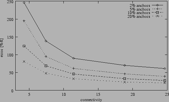 |
Figure 2 shows the average performance of
the Hop-TERRAIN algorithm as a function of connectivity and anchor
population in the presence of 5% range errors. As seen in this plot,
position estimates by Hop-TERRAIN have an average accuracy under 100%
error in scenarios with at least 5% anchor population and an average
connectivity level of 7 or greater. In extreme situations where very few
anchors exist and connectivity in the network is very low, Hop-TERRAIN
errors reach above 250%.
Figure 3:
Average position error after Refinement (5% range errors).
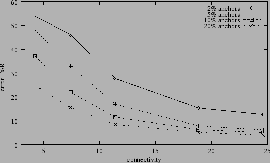 |
Figure 4:
Fraction of located nodes (2% anchors, 5% range errors).
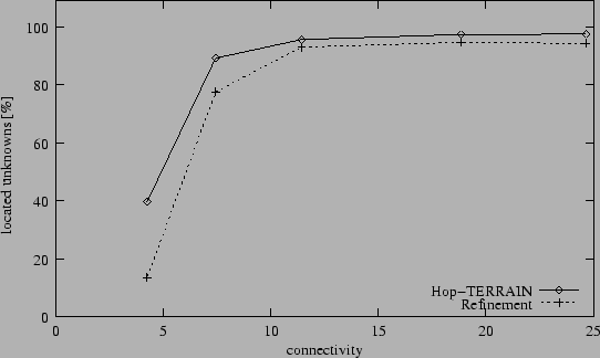 |
Figure 3 displays the results from the same experiment
depicted in Figure 2, but now the position estimates
of Hop-TERRAIN are subsequently processed by the Refinement algorithm.
Its shape is similar to that of Figure 2, showing
relatively consistent error levels of less than 33% in scenarios with
at least 5% anchor population and an average connectivity level of
7 or greater. Refinement also has problems with low connectivity and
anchor populations, and is shown to climb above 50% position error in
these harsh conditions. Overall Refinement improves the accuracy of the
position estimates by Hop-TERRAIN by a factor three to five.
Figure 4 helps to explain the sharp increases in
positioning errors for low anchor populations and sparse networks
shown in figures 2 and 3.
Figure 4 shows that, as the average connectivity
between nodes throughout the network decreases past certain points,
both algorithms break down, failing to derive position estimates for
large fractions of the network. This is due simply to a lacking of
sufficient information, and is a necessary consequence of loosely
connected networks. Nodes can only be located when connected to at
least 3(4) neighbors; Refinement also requires a minimal confidence level
(0.1). It should be noted that the results in Figure 4
imply that the reported average position errors for low connectivities in
figures 2 and 3 have low statistical
significance, as these points represent only small fractions of the
total network. Nevertheless, the general conclusion to be drawn from
figures 2, 3, and 4
is that both Hop-TERRAIN and Refinement perform poorly in networks with
average connectivity levels of less than 7.
Figure 5:
Average position error after Hop-TERRAIN (2D grid,
5% range errors).
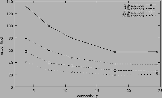 |
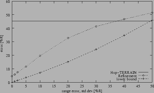
Figure 6:
Range error sensitivity (10% anchors, connectivity 12).
 |
Since connectivity has a pronounced effect on position error we were
interested if other topological characteristics would show large effects
as well. In the following
experiment we randomly place 400 nodes on the vertices of a 200x200
grid, rather than allowing the nodes to sit anywhere in the square
area. We found that the grid layout did
not result in better performance for the Refinement algorithm, relative to
the performance of the Refinement algorithm with random node placement.
We do not include a plot here because it looks almost identical to
Figure 3. We did find a difference in performance
for Hop-TERRAIN though. Figure 5 shows that placing
the nodes on a grid dramatically reduces the errors of the Hop-TERRAIN
algorithm in the cases where connectivity or anchor node populations are
low. For example, with 5% anchors and a connectivity of 8 nodes, the
average position error decreases from 95% (random distribution) to 60%
(grid). We suspect this is due to the consistent distances between nodes,
the ideal topologies within clusters that result form the grid layout, and
the inherently optimized connectivity levels across the entire network.
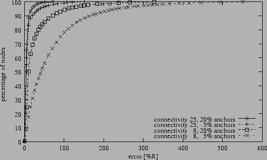
Figure 7:
Cumulative error distribution (5% range errors).
 |
Sensitivity to average error levels in the range measurements is a
major concern for positioning algorithms. Figure 6
shows the results of an experiment in which we held anchor population
and connectivity constant at 10% and 12 nodes, respectively, while
varying the average level of error in the range measurements. We found
that Hop-TERRAIN was almost completely insensitive to range errors.
This is a result of the binary nature of the procedure in which routing
hops are counted; if nodes can see each other, they pass on incremented
hop counts, but at no time do any nodes attempt to measure the actual
ranges between them. Unlike Hop-TERRAIN, Refinement does rely on the
range measurements performed between nodes, and Figure 6
shows this dependence accordingly. At less than 40% error in the range
measurements, on average, Refinement offers improved position estimates
over Hop-TERRAIN. The results improve steadily as the
range errors decrease. For reference we determined the best possible
position information that can be obtained in each case. For each node we
performed a triangulation using the true positions of its neighbors
and the corresponding erroneous range measurements. The resulting position
errors are plotted as the lower bound in Figure 6. This
suggests that there is room for improvement for Refinement.
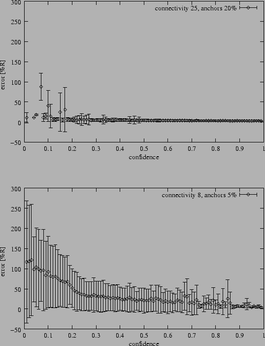
Figure 8:
Relation between confidence and positioning error (average and
standard deviation).
 |
Up until this point we reported average position errors.
Figure 7, in contrast, gives a detailed look at the
distribution of the position errors for individual nodes under four
different scenarios. Note that the distributions have similar shapes:
many nodes with small errors, large tails with outliers. Refinement's
confidence metrics are to some extent capable of pinpointing the
outliers. Figure 8 shows the relationship between
position error levels and the corresponding confidence values assigned
to each node. The data for Figure 8 was taken from the
best and worst case scenarios from the same experiment used to generate
Figure 7. As desired, the nodes with higher position
errors are assigned lower confidence levels. In the easier case, the
confidence indicators are much more reliable than in the more difficult
case. The large standard deviations, however, show that confidence is not
a good indicator for position accuracy. This is unfortunate
since a reliable confidence metric would be very useful for applications,
for example, to identify regions of ``bad'' nodes. Currently, the value
of using confidence levels is the improved average positioning error
compared to a naive implementation of Refinement without confidences.
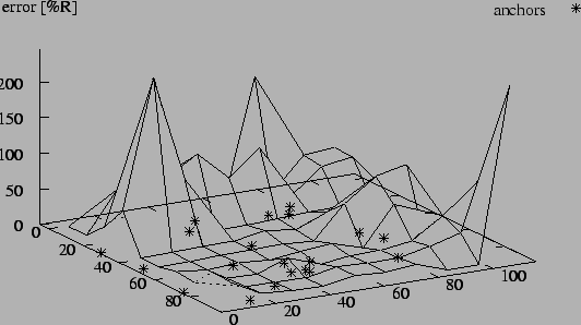
Finally, yet another useful way of looking at the distribution of errors
over individual nodes is to take their geographical location into account.
Figure 9 plots positioning errors as a function of a node's
location in the square testing area. This experiment used 400 randomly
placed nodes, an anchor population of 5%, an average connectivity
level of 12, and range errors of 5%. The error distribution in
Figure 9 is quite typical for many scenarios showing that
areas along the edges of the network lacking a high concentration of
anchor nodes are particularly susceptible to high position errors.
Discussion
Figure 9:
Geographic error distribution (5% anchors, connectivity 12, 5% range
errors).
 |
It is interesting to compare our results from the previous section with
the alternative approaches discussed in Section 2. First,
we discuss the performance of Hop-TERRAIN and related algorithms that do
not use range measurements. Hop-TERRAIN is similar to the ``DV-hop''
algorithm by Niculescu and Nath [10], but we get
consistently higher position errors, for example, 69% (Hop-TERRAIN)
versus 35% (DV-hop) on a scenario with 10% anchors and a connectivity
of 8. Under poorer network conditions though, Hop-TERRAIN is more
robust than DV-hop, showing about a factor of 2 improvement in position
accuracy in sparsely connected networks. Regardless, the trend observed
in both studies is the same: when the fraction of anchors drops below 5%,
position errors rapidly increase. The convex optimization technique by
Doherty et al. [5] is about as accurate as Hop-TERRAIN,
except for very low fractions of anchors. For example, convex optimization
achieves position errors that are above 150% on a scenario (200 nodes,
5% anchors, connectivity of 6) where Hop-TERRAIN errors are around 125%;
the gap grows for even lower fractions of anchors. As mentioned earlier,
convex optimization is a centralized algorithm.
The results of Refinement are comparable to those reported by Savvides
et al. for an ``iterative multilateration'' scenario with 50 nodes, 20%
anchors, connectivity 10, and 1% range errors [12]. Their
algorithm, however, can handle neither low anchor fractions nor low
connectivities, because positioning starts from nodes connected to at
least 3 anchors. Refinement still performs acceptably well with few
anchors or a low connectivity. Furthermore the preliminary results of
their more advanced ``collaborative multilateration'' algorithm show
that Refinement is able to determine the position of a larger fraction of
unknowns: 56% (Refinement) versus 10% (collaborative multilateration)
on a scenario with just 5% anchors (200 nodes, connectivity 6).
The ``Euclidean'' algorithm by Niculescu and Nath uses range
estimates to construct local maps that are unified into a single
global map [10]. The results reported for random
configurations show that ``Euclidean'' is rather sensitive to range
errors, especially with low fractions of anchors: in case of 10% anchors
their Hop-TERRAIN equivalent (DV-hop) outperforms Euclidean. Refinement
achieves better position estimates and is more robust since
the cross over with Hop-TERRAIN occurs around 40% range errors (see
Figure 6).
In summary, the performance of Hop-TERRAIN and Refinement is comparable
to other algorithms in the case of ``easy'' network topologies (high
connectivity, many anchors) with low range errors, and outperforms the
competition in difficult cases (low connectivity, few anchors, large
range errors). The results of refinement can most likely be improved even
further when the placement of anchors nodes can be controlled given the
positive experience reported by others [2,5].
Since the largest errors occur along the edges of the network (see
Figure 9), most anchors should be placed on the perimeter
of the network. Another approach to increase the accuracy of locationing
systems is to use other sources of information. When locating sensors in a
room, for example, knowing that the sensors are wall mounted eliminates
one degree of freedom. Incorporating such knowledge in localization
algorithms, however, requires great care. For example, knowing that
two sensors cannot communicate does not imply that they are located far
apart since a wall may simply prohibit radio communication.
Based on the experimental results from Section 5 and the
discussion above we recommend a number of guidelines for the installation
of wireless sensor networks:
-
- place anchors carefully (i.e. at the edges), and either
-
- ensure a high connectivity ( 10), or
-
- employ a reasonable fraction of anchors ( 5%).
This will create the best conditions for positioning algorithms in general, and
for Hop-TERRAIN and Refinement in particular.
Conclusions and future work
In this paper we have presented a completely distributed algorithm
for solving the problem of positioning nodes within an ad-hoc,
wireless network of sensor nodes. The procedure is partitioned
into two algorithms: Hop-TERRAIN and Refinement. Each algorithm is
described in detail. The simulation environment used to evaluate
these algorithms is explained, including details about the specific
implementation of each algorithm. Many experiments are documented for
each algorithm, showing several aspects of the performance achieved
under many different scenarios. The results show that we are able to achieve
position errors of less than 33% in a scenario with 5% range measurement
error, 5% anchor population, and an average connectivity of 7 nodes.
Finally, guidelines for implementing and deploying a network that will
use these algorithms are given and explained.
An important aspect of wireless sensor networks is energy consumption.
In the near future we therefore plan to study the amount of communication
and computation induced by running Hop-TERRAIN and Refinement. A
particularly interesting aspect is how the accuracy vs. energy
consumption trade-off changes over subsequent iterations of Refinement.
We would like to thank DARPA for funding the Berkeley Wireless Research
Center under the PAC-C program (Grant #F29601-99-1-0169). Also, Koen
Langendoen was supported by the USENIX Research Exchange (ReX) program,
which allowed him to visit the BWRC for the summer of 2001 and work on
the Refinement algorithm. Finally, we would like to thank the anonymous
reviewers and our ``shepherd'' Mike Spreitzer for their constructive
comments on the draft version of this paper.
- 1
-
J. Beutel.
Geolocation in a Pico Radio environment.
Master's thesis, ETH Zürich, December 1999.
- 2
-
N. Bulusu, J. Heidemann, V. Bychkovskiy, and D. Estrin.
Density-adaptive beacon placement algorithms for localization in ad
hoc wireless networks.
In IEEE Infocom 2002, New York, NY, June 2002.
- 3
-
N. Bulusu, J. Heidemann, and D. Estrin.
GPS-less low-cost outdoor localization for very small devices.
IEEE Personal Communications, 7(5):28-34, Oct 2000.
- 4
-
S. Capkun, M. Hamdi, and J.-P. Hubaux.
GPS-free positioning in mobile ad-hoc networks.
In Hawaii Int. Conf. on System Sciences (HICSS-34), pages
3481-3490, Maui, Hawaii, January 2001.
- 5
-
L. Doherty, K. Pister, and L. El Ghaoui.
Convex position estimation in wireless sensor networks.
In IEEE Infocom 2001, Anchorage, AK, April 2001.
- 6
-
L. Girod and D. Estrin.
Robust range estimation using acoustic and multimodal sensing.
In IEEE/RSJ Int. Conf. on Intelligent Robots and Systems
(IROS), Maui, Hawaii, October 2001.
- 7
-
J. Hightower and G. Borriello.
Location systems for ubiquitous computing.
IEEE Computer, 34(8):57-66, Aug 2001.
- 8
-
J. Hightower, R. Want, and G. Borriello.
SpotON: An indoor 3D location sensing technology based on RF
signal strength.
UW CSE 00-02-02, University of Washington, Department of Computer
Science and Engineering, Seattle, WA, February 2000.
- 9
-
R. Mukai, R. Hudson, G. Pottie, and K. Yao.
A protocol for distributed node location.
IEEE Communication Letters, to be published.
- 10
-
D. Niculescu and B. Nath.
Ad-hoc positioning system.
In IEEE GlobeCom, November 2001.
- 11
-
C. Savarese, J. Rabaey, and J. Beutel.
Locationing in distributed ad-hoc wireless sensor networks.
In IEEE Int. Conf. on Acoustics, Speech, and Signal Processing
(ICASSP), pages 2037-2040, Salt Lake City, UT, May 2001.
- 12
-
A. Savvides, C.-C. Han, and M. Srivastava.
Dynamic fine-grained localization in ad-hoc networks of sensors.
In 7th ACM Int. Conf. on Mobile Computing and Networking
(Mobicom), pages 166-179, Rome, Italy, July 2001.
- 13
-
A. Varga.
The OMNeT++ discrete event simulation system.
In European Simulation Multiconference (ESM'2001), Prague,
Czech Republic, June 2001.
Robust Positioning Algorithms for Distributed Ad-Hoc Wireless Sensor Networks
This document was generated using the
LaTeX2HTML translator Version 99.2beta6 (1.42)
Copyright © 1993, 1994, 1995, 1996,
Nikos Drakos,
Computer Based Learning Unit, University of Leeds.
Copyright © 1997, 1998, 1999,
Ross Moore,
Mathematics Department, Macquarie University, Sydney.
The command line arguments were:
latex2html -split 0 robust-positioning.tex
The translation was initiated by Koen Langendoen on 2002-04-16
Footnotes
- ... mean1
- Ranges
are enforced to be non-negative by clipping values below zero.
Koen Langendoen
2002-04-16
|
