Similar to the idealistic model described in Section
4.1, the location of the observer can be obtained by
determining the intersection point(s) of the three rotational
hyperboloids defined by Equation 9. However, since the
observed virtual beam width ![]() now additionally depends on the height
now additionally depends on the height
![]() of the observer, we have to take into account the exact lighthouse
positions. Figure 6, which shows an extended
version of Figure 3, illustrates this. The marks on
the coordinate axes show the positions of the lighthouse center (as
defined in Section 4.2.2) of each of the three
lighthouses. That is, the coordinates of the observer are
of the observer, we have to take into account the exact lighthouse
positions. Figure 6, which shows an extended
version of Figure 3, illustrates this. The marks on
the coordinate axes show the positions of the lighthouse center (as
defined in Section 4.2.2) of each of the three
lighthouses. That is, the coordinates of the observer are
![]() with respect to the origin formed by the
intersection of the three lighthouse rotation axes. In order to obtain
approximations for the values
with respect to the origin formed by the
intersection of the three lighthouse rotation axes. In order to obtain
approximations for the values ![]() ,
, ![]() , and
, and ![]() , we have to
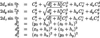
solve the following equation system:
, we have to
solve the following equation system:
The indices ![]() indicate which lighthouse the values are
associated with. As with equation system 4, this system does
not necessarily have a solution, since the parameters are only
approximations obtained by measurements. Therefore, minimum mean
square error (MMSE) methods have to be used to obtain approximations
for the
indicate which lighthouse the values are
associated with. As with equation system 4, this system does
not necessarily have a solution, since the parameters are only
approximations obtained by measurements. Therefore, minimum mean
square error (MMSE) methods have to be used to obtain approximations
for the ![]() . However, if the equation system 10
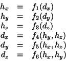
has a solution, we can approximately solve it by simple iteration. For
this, we first transform each of the six equations of equation system
10 in order to obtain the following fixpoint form:
. However, if the equation system 10
has a solution, we can approximately solve it by simple iteration. For
this, we first transform each of the six equations of equation system
10 in order to obtain the following fixpoint form:
Note that we did not show arguments of the ![]() (i.e.,
(i.e.,
![]() ,
,
![]() ) that do not change
during iterative evaluation of the equation system. By using
appropriate values for
) that do not change
during iterative evaluation of the equation system. By using
appropriate values for
![]() , and
, and ![]() , we can
obtain approximate solutions for
, we can
obtain approximate solutions for ![]() with the following
algorithm:
with the following
algorithm:


while (true) {
if (
) break;


}
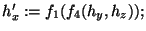
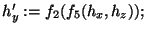
At first, the ![]() are initialized to the start values
are initialized to the start values
![]() . Using the
. Using the ![]() , new approximations
, new approximations ![]() are
computed. We are finished if the new values are reasonably close to
the original
are
computed. We are finished if the new values are reasonably close to
the original ![]() . Otherwise we update the
. Otherwise we update the ![]() to the new
values and do another iteration. For good convergence of this
algorithm the partial derivatives of the
to the new
values and do another iteration. For good convergence of this
algorithm the partial derivatives of the
![]() in the
environment of the solution
in the
environment of the solution
![]() should be small, which
is typically true. In our prototype implementation we use
should be small, which
is typically true. In our prototype implementation we use
![]() cm and
cm and ![]() cm. With this configuration, the algorithm
typically performs 4-6 iterations.
cm. With this configuration, the algorithm
typically performs 4-6 iterations.
![\includegraphics[width=6cm]{loc-system2}](img70.gif)