|
WiTMeMo '05 Paper
[WiTMeMo '05 Technical Program]


Mobility Assessment for MANETs Requiring Persistent Links
| Sanlin Xu |
Kim Blackmore |
Haley Jones |
| Department of Engineering, Australian National University |
Mobile ad hoc networks (MANETs) have inherently dynamic
topologies. It is important to be able to determine the
reliability of the communication paths created under these
difficult circumstances. For this purpose, mobility metrics have
been proposed in the literature, but most existing research is
based on simulation results and empirical analysis. We consider
two metrics, link persistence and path persistence, and develop an
analytical framework to derive their exact expressions as well as
the corresponding link residual time and path residual time, under
a random mobility environment. Such exact expressions constitute
precise mathematical relationships between the network
connectivity and the mobility of mobile nodes. This framework
could be used to develop efficient algorithms for medium access
control, or to optimize existing network routing protocols.
1 Introduction
Mobile ad hoc networks are comprised of
mobile nodes communicating via wireless links. Due to the
mobility, communication paths are dynamic, affecting path
reliability. Meaningful analysis of the reliability of these
constituent links is crucial to understanding the reliability of
the paths themselves. Node mobility leads to changes in network
topology resulting in link additions and breakages, and alteration
of traffic patterns and/or traffic distributions. Routing
protocols [12,11,9] based on mobility
metric prediction have been shown to increase the packet delivery
ratio and reduce routing overhead.
In this paper, we consider the notions of link
persistence and path persistence to describe the
continuous link and path availabilities, respectively, for an
active communication route. The link (path) persistence is the
probability that a link (path) lasts constantly until a future
time,  , given that it existed at time 0
. From theoretical
analyses of the link (path) persistence, we derive the expected
residual time for an active link (path). The residual time is
evaluated deterministically in [12,11], by
simulation in [4,2,10], and by
calculation in [13]. Note that the various mobility
measures have been given different names by different authors.
, given that it existed at time 0
. From theoretical
analyses of the link (path) persistence, we derive the expected
residual time for an active link (path). The residual time is
evaluated deterministically in [12,11], by
simulation in [4,2,10], and by
calculation in [13]. Note that the various mobility
measures have been given different names by different authors.
A similar measure to link persistence, link availability, is
considered by Jiang et al [6]. The link
availability is approximated as the ratio of the mean time a link
will be continuously available to a link prediction time. The
calculation method in [6] relies on a parameter,
 , that must be experimentally determined. In
[8], link availability is also considered but, in
this case, a link is considered to be available at
even if it
has undergone failure during the time between 0 and
. Further,
in [13] an expression for link availability, using a
simple straight line mobility model, is derived.
, that must be experimentally determined. In
[8], link availability is also considered but, in
this case, a link is considered to be available at
even if it
has undergone failure during the time between 0 and
. Further,
in [13] an expression for link availability, using a
simple straight line mobility model, is derived.
Our notion of link or path persistence requires a random mobility
model [3] governing the behaviour of the nodes in the
network. We assume nodes move according to a generalisation of the
Random Walk Mobility Model. Such an assumption is clearly not
realistic, but may be useful as an aid to predicting link
reliability for routing purposes [8]. Moreover,
random mobility models are regularly used for protocol evaluation
[2], so our work is important to facilitate comparison
of the evaluation environment with practical implementation
environments.
This paper is organised as follows. In
Section 2 we present definitions for the
mobility metrics investigated in this paper. In
Section 3 we develop an expression for
the PDF of the separation distance between an arbitrary pair of
mobile nodes after one epoch, and generalize the results to a
network of nodes with i.i.d. mobility. In
Section 4 we develop a Markov chain
model for the evolution of the separation distance between two
nodes. This Markov model is applied, in
Section 5, to the determination of expressions
for a range of mobility metrics. In Section 6
we compare our theoretical and simulation results. Finally, we
present conclusions in Section 7.
2 Mobility Metric Definitions
While fading links are the norm in
wireless communication networks [7], the existing
literature on mobility in MANETs concentrates on ``binary'' links.
That is, links are understood to be ``on'' or ``off'' at any point
in time. Schemes which use network topology information are
sensitive to the length of time for which a link is consistently
``on''. Therefore, we consider the following metrics, which assume
that the link is ``on'', and ask how long it will continue to be
``on''.
- Link Persistence,
 : Given an active
link between two nodes at time 0, the persistence of this link,
, until (at least) epoch
is defined as the
probability that the link continuously lasts until epoch
.
: Given an active
link between two nodes at time 0, the persistence of this link,
, until (at least) epoch
is defined as the
probability that the link continuously lasts until epoch
.
 Lasts until Lasts until Available at Available at |
(1) |
- Link Residual Time,
 : Given an active link
between two nodes at time 0, the link residual
time,
, is
the length of time for which the link will
continue to exist until it is broken.
: Given an active link
between two nodes at time 0, the link residual
time,
, is
the length of time for which the link will
continue to exist until it is broken.
- Path Persistence,
 : Given an
active path with
: Given an
active path with  hops between two nodes at time 0,
the path persistence, at epoch
, is defined as
the probability that the path will continuously last until at
least epoch
.
hops between two nodes at time 0,
the path persistence, at epoch
, is defined as
the probability that the path will continuously last until at
least epoch
.
 Last untilAvailable at Last untilAvailable at |
(2) |
- Path Residual Time,
 : Given an active
path with
hops between two nodes at
time 0, the path residual time,
, is the length of time for which the path will
continue to exist.
: Given an active
path with
hops between two nodes at
time 0, the path residual time,
, is the length of time for which the path will
continue to exist.
3 Node Separation After One Epoch
In this paper, we assume that each
mobile node moves with a velocity uniformly distributed in both
speed,  , and direction,
  . Both the speed and direction
change in each epoch but are constant for the duration of an
epoch, and independent of each other. The speed has mean,
. Both the speed and direction
change in each epoch but are constant for the duration of an
epoch, and independent of each other. The speed has mean,
 , and variance
 , such that
 . The direction,
, is uniformly distributed in
. The direction,
, is uniformly distributed in  . This random
mobility model is widely used to analyze route stability in
multi-hop mobile environments [11,13,1].
. This random
mobility model is widely used to analyze route stability in
multi-hop mobile environments [11,13,1].
The status of a wireless link depends on numerous system and
environmental factors that affect transmitter and receiver
transmission range. A widely applied, albeit optimistic, model is
used in this paper, whereby transmission range is approximated by
a circle of radius  corresponding to a signal strength
threshold. If the separation distance between a given pair of
nodes is less than
, it is assumed the link between them is
active. Let the random variable representing the separation
distance between two nodes at epoch
corresponding to a signal strength
threshold. If the separation distance between a given pair of
nodes is less than
, it is assumed the link between them is
active. Let the random variable representing the separation
distance between two nodes at epoch  be
be  , and let
  denote an instance of
. The PDF,
denote an instance of
. The PDF,
 , forms a basis for the derivations
of expressions for the metrics given in
Section 2. We derive this PDF below.
, forms a basis for the derivations
of expressions for the metrics given in
Section 2. We derive this PDF below.
3.1 Relative Movement Between  Nodes
Nodes
To determine
, we begin with the PDF
of the relative movement between a given pair of nodes,
labelled  and
and  . The relationship between the relative
movement vector,
. The relationship between the relative
movement vector,
 , in any given epoch, and the
node velocity vectors,
, in any given epoch, and the
node velocity vectors,
 and
and
 , is
, is
 , as depicted in
Fig. 1. Let
, as depicted in
Fig. 1. Let  be the random variable representing
the magnitude of
, similarly for
be the random variable representing
the magnitude of
, similarly for  and
and
 . Let
. Let  be the angle between
and
. As
be the angle between
and
. As
 , we use the Jacobian transform
to obtain the joint PDF:
, we use the Jacobian transform
to obtain the joint PDF:
Figure 1:
Relationship between the node movement vectors
 and
and
 of nodes
and
,
relative movement vector,
, initial
separation distance,
, and separation vector,
of nodes
and
,
relative movement vector,
, initial
separation distance,
, and separation vector,
 .
.
|
As
is uniformly distributed in  and
,
and
are independent, we can simplify
(3) to
and
,
and
are independent, we can simplify
(3) to
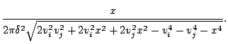
Then the marginal PDF of the magnitude of the relative movement
is,
 |
(5) |
Thus, (4) and (5) describe the
behaviour of the relative distance,
, between a given pair of
nodes,
and
, in any one epoch.
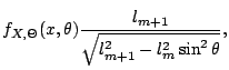
From Fig. 1,
=
 +
. Let
+
. Let  from
Fig. 1 be uniformly distributed in the interval
. The conditional PDF is
from
Fig. 1 be uniformly distributed in the interval
. The conditional PDF is
where
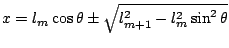 .
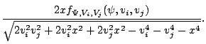
Since the magnitude and phase are independent, we obtain
.
Since the magnitude and phase are independent, we obtain
 |
(7) |
where
 , due to the triangular
relationship between
,
and
.
, due to the triangular
relationship between
,
and
.
Next, we use
to derive the node
separation distance PDF after
epochs.
4 Markov Chain Model of Separation
In Section ![[*]](crossref.png) we derived the PDF of the distance between a given pair of
nodes in epoch we derived the PDF of the distance between a given pair of
nodes in epoch  ,
,  , given the separation distance in
epoch
. That is, the separation distance in epoch
can be
represented as a random variable,
. The evolution of the
separation distance can be represented by a sequence of random
variables,
, given the separation distance in
epoch
. That is, the separation distance in epoch
can be
represented as a random variable,
. The evolution of the
separation distance can be represented by a sequence of random
variables,
 . So, the
relationship between the separation distances in a sequence of
epochs readily lends itself to modelling via a Markov chain
process.
. So, the
relationship between the separation distances in a sequence of
epochs readily lends itself to modelling via a Markov chain
process.
4.1 Transition Model
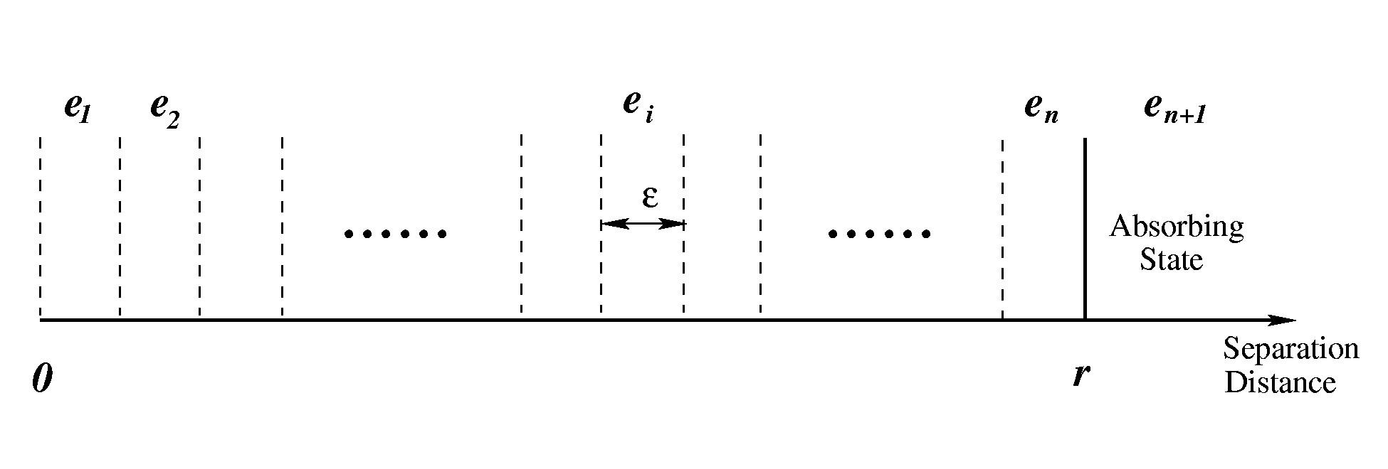
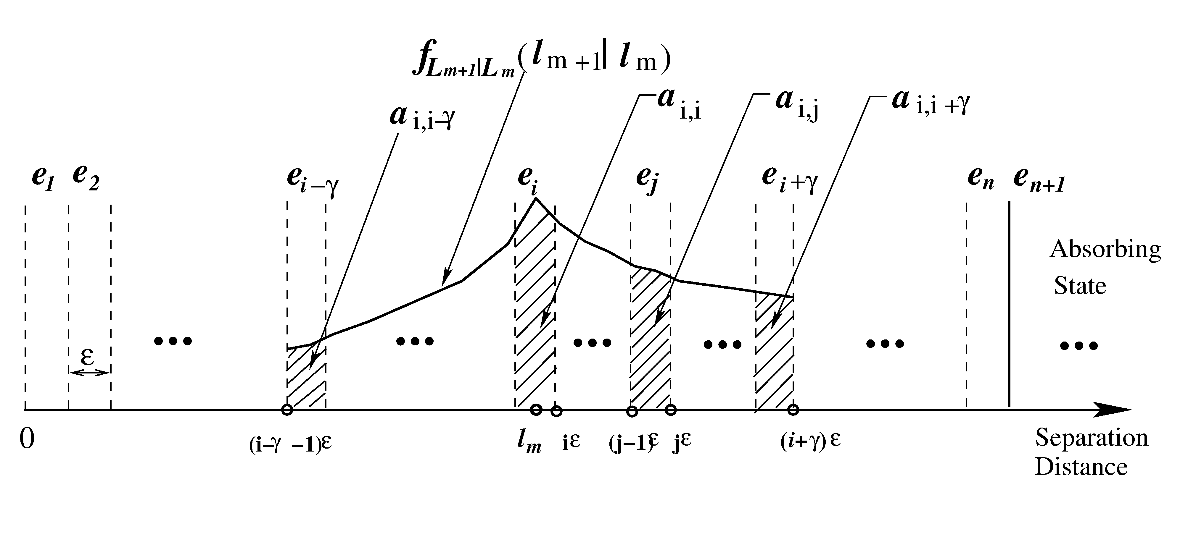
Figure 2:
State space for distance between a pair of nodes, where
separations outside of the transmission range (absorbing state) result in a link being
discarded.
|
We first define the state space governing the range of node
separation distances,
 . We divide the interval
 into
into  bins of width
. If a link is active,
falls into one of these bins, as shown in
Fig. 2. The
th bin corresponds to the
th state, denoted
bins of width
. If a link is active,
falls into one of these bins, as shown in
Fig. 2. The
th bin corresponds to the
th state, denoted  . The
. The  th state, corresponding to
 , is defined as the absorbing state. A separation
distance in the absorbing state indicates a broken link. If the
nodes move back within communication range, a new link is
considered to have been formed. The distance,
, is in
if the following conditions hold,
, is defined as the absorbing state. A separation
distance in the absorbing state indicates a broken link. If the
nodes move back within communication range, a new link is
considered to have been formed. The distance,
, is in
if the following conditions hold,
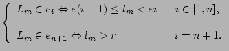 |
(8) |
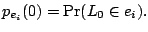
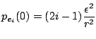
4.2 Initial Condition Vector
The initial condition vector denotes the probability of the
initial separation distance,  , being in each state at time 0.
It has entries
, being in each state at time 0.
It has entries
 |
(9) |
We assume nodes are initially uniformly distributed. Since they
move according to a random walk, they remain (approximately)
uniformly distributed in the transmission region. Therefore, if a
link exists the initial separation distance,
, has a linear
distribution [5]:
 , , |
(10) |
 , , |
(11) |
Figure 3:
Shows  , the probability of transferring from
to
, the probability of transferring from
to  after one epoch, for various
.
after one epoch, for various
.
|
Let
be in
. Then, after one epoch,  , must be
in the range
, must be
in the range
![$ [l_m-2(\overline{v}+\delta),l_m+2(\overline{v}+\delta)]$](img79.png) . This
corresponds to
being in
such that
. This
corresponds to
being in
such that
![$ j \in
[\max(1,i-\gamma), \min(i+\gamma,n+1)]$](img80.png) , where
, where
 , is the maximum number
of bins that can be traversed in a single epoch. The transition
matrix is denoted by
, is the maximum number
of bins that can be traversed in a single epoch. The transition
matrix is denoted by
![$\displaystyle A = \left[
\begin{array}{cccc}
a_{11} & \cdots & a_{1,n} & a_{1...
...& \cdots & a_{n,n} &a_{n,n+1}
0 & \cdots &0 & 1
\end{array}
\right],$](img82.png) |
(12) |
where
is the probability of transition from
to
in a given epoch. We note that
 and
and
 . The last row in (12)
represents transition from absorbing state.
. The last row in (12)
represents transition from absorbing state.
To calculate the transition probabilities between non-absorbing
states, illustrated in Fig. 3, consider the
state transition probabilities at epoch
, and using
(7)
The PDF
 changes with
. However, if
is sufficiently small, and
is known, we can assume
that
is approximately uniformly distributed within the
th
bin. In this case,
changes with
. However, if
is sufficiently small, and
is known, we can assume
that
is approximately uniformly distributed within the
th
bin. In this case,
 |
(14) |
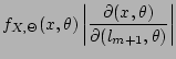
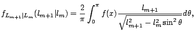
Moreover, we can approximate the PDF of the conditioned separation
distance from any point in
to any point in
using the
midpoints of the two states:
![$\displaystyle f_{L_{m+1}\vert L_m}(l_{m+1}\vert l_m)
\approx
f_{L_{m+1}\vert L_m}\left [(j-1/2)\varepsilon \vert (i-1/2)\varepsilon \right ].$](img90.png) |
(15) |
Thus, from (13), (14) and
(15) we can write
![$\displaystyle a_{ij}
\approx
\varepsilon f_{L_{m+1}\vert L_m}\left[(j-1/2)\varepsilon\vert(i-1/2)\varepsilon\right].$](img91.png) |
(16) |
4.4 Distribution After
Epochs
According to the properties of Markov
Chains, we can use  and
and  to determine the probability of
the separation distance being in state
after
epochs:
to determine the probability of
the separation distance being in state
after
epochs:
![$\displaystyle P(k) = [p_{e_1}(k) p_{e_2}(k) \cdots p_{e_{n+1}}(k)] = P(0) A^k,$](img94.png) |
(17) |
5 Mobility Metric Calculations
Having developed a Markov chain model for
the evolution of the node separation, we now derive expressions
for the mobility metrics defined in Section 2.
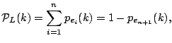
The probability of the link being in existence after
epochs is
the probability that the separation distance is in a
non-absorbing state:
 |
(18) |
where
 can be calculated from (17).
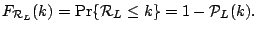
The CDF,
 , of the link residual time, is:
 |
(19) |
Then, the PDF of the link residual time is
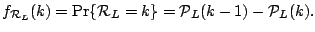 |
(20) |
The expected value of the link residual time is
![$\displaystyle E\{\mathcal{R}_L\}
= \sum_{k=1}^{\infty} k f_{\mathcal{R}_L}(k)
= \sum_{k=1}^{\infty}k [\mathcal{P}_{L}(k-1)-\mathcal{P}_{L}(k)].$](img100.png) |
(21) |
For a path to persist, each of the component links must persist:
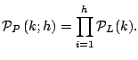 |
(22) |
The CDF,
 , of the path residual time is
 |
(23) |
Therefore, the PDF of the path residual time is
 |
(24) |
And, the expected value of the path residual time is
![$\displaystyle E\{\mathcal{R}_P(h)\}
=
\sum_{k=1}^{\infty}k [\mathcal{P}_{P}(k-1;h)-\mathcal{P}_{P}(k;h)].$](img106.png) |
(25) |
6 Simulation Results
We verify all analytically derived
expressions for the mobility metrics by simulation. The
simulations were conducted with MNs moving according to the
description in Section 3.
The network consisted of  nodes initially placed randomly in
a square plane of side
nodes initially placed randomly in
a square plane of side  distance units. We use the generic
term ``units'' rather than, say, m or km because it is the
relative and not the absolute distances that are important. Each
MN had a maximum transmission range of
distance units. We use the generic
term ``units'' rather than, say, m or km because it is the
relative and not the absolute distances that are important. Each
MN had a maximum transmission range of  units, with between
and
units, with between
and  epochs per trial for
  trials.
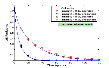
Figure 6 illustrates the comparisons of
the simulation results to the theoretical calculations. The link
persistence, shown in Fig. 4(a), decreases with
increasing simulation time and, at a greater rate with increasing
ratio of mean node speed to transmission range,
 .
Further, the path persistence drops off at a greater rate than the
link persistence, for the same mean node speed, as would be
expected. The path persistence also drops off more quickly with an
increased number of hops, as there is more chance of an individual
link breaking.
.
Further, the path persistence drops off at a greater rate than the
link persistence, for the same mean node speed, as would be
expected. The path persistence also drops off more quickly with an
increased number of hops, as there is more chance of an individual
link breaking.
In the bounded simulation environment, MNs were ``reflected'' back
into the simulation area, if their movement would otherwise take
them outside. Consequently, nodes near the edge are more likely to
remain in transmission range, and the link persistence is
artificially increased, compared to that for the unbounded
simulation area. The experimental results for the bounded area are
still close to the calculated results, as expected, though not as
well matched.
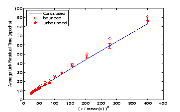
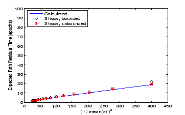
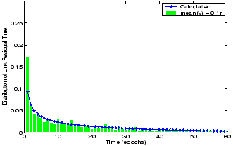
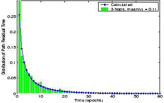
The expected link and path residual times have been plotted
against the second order of
 , each showing a
linear relationship, particularly for larger ratios. As expected,
, each showing a
linear relationship, particularly for larger ratios. As expected,
 is much lower than
 for
the same communication range to speed ratio. Finally, the
probability distributions of
and
for
the same communication range to speed ratio. Finally, the
probability distributions of
and
 show that the path residual time is more likely to have a shorter
length, in epochs, than the link residual time.
show that the path residual time is more likely to have a shorter
length, in epochs, than the link residual time.
Figure 4:
Comparison of the mobility metric calculations and
simulated results. Each MN moves at a randomly chosen velocity
during each epoch, which has uniformly distributed speed with
mean
, and uniformly distributed direction in
the range
. The ``shape'' plots in each figure indicate simulated
results, while the solid lines indicate calculated values with the
relevant equations within the paper. The vertical bar indicates the  confidence
interval for the unbounded scenario.
confidence
interval for the unbounded scenario.
[a]
 [b]
[b]
 [c]
[c]
 [d]
[d]
 [e]
[e]
 [f]
[f]
|
7 Conclusions
Frequent changes in network topology
caused by mobility in MANETs imposes great challenges for
developing efficient routing algorithms. The theoretical analysis
framework presented in this paper provides a better understanding
of network behavior under mobility and some fundamental work on
the issue of path stability. We propose link persistence and path
persistence for evaluating link and path stability. The Markov
chain model used in this paper, has enabled us to accurately
determine a series of mobility metrics. These calculations are
useful for comparison of artificial mobility behaviours with
actual network implementation scenarios. The analytical results
can be readily applied to various adaptive routing protocols that
use corresponding mobility metrics.
- 1
-
B. An and S. Papavassiliou.
An Entropy-Based Model for Supporting and Evaluating
Route Stability in Mobile Ad Hoc Wireless Networks.
IEEE Commun. Lett., 6(8):328-330, 2002.
- 2
-
F. Bai, N. Sadagopan, and A. Helmy.
IMPORTANT a Framework to Systematically Analyze the Impact
of Mobility on Performance of Routing Protocols for Ad Hoc
Networks.
In IEEE INFOCOM, volume 2, pages 825-835, April 2003.
- 3
-
T. Camp, J. Boleng, and V. Davies.
A Survey of Mobility Models for Ad Hoc Network
Research.
Wireless Commun. and Mobile Computing (WCMC), 5(2):483-502,
2002.
- 4
-
M. Gerharz, C. Waal, and P. Martini.
Strategies for Finding Stable Paths in Mobile Wireless
Ad Hoc Networks.
In Proc. of IEEE Conf. on Local Computer Networks (LCN), pages
130-139, October 2003.
- 5
-
D. Hong and S. Rappaport.
Traffic Model and Performance Analysis for Cellular
Mobile Radio Telephone Systmes with Prioritized and
Nonprioritized Handoff Procedures.
IEEE Trans. Veh. Technol., 35:77-92, August 1986.
- 6
-
S. Jiang.
An Enhanced Prediction-based Link Availability Estimation
for Manets.
IEEE Trans. Commun., 52(2):183-186, February 2004.
- 7
-
H. Jones, S. Xu, and K. Blackmore.
Link Ratio for Ad Hoc Networks in a Rayleigh Fading
Channel.
WITSP, Australia, December 2004.
- 8
-
A. B. McDonald and T. Znati.
A Mobility Based Framework for Adaptive Clustering in
Wireless Ad-Hoc Networks.
IEEE J. Select. Areas Commun., 17(8):1466-1487, August 1999.
- 9
-
L. Qin and T. Kunz.
Increasing Packet Delivery Ratio in DSR by Link
Prediction.
In Proc. 36th Hawaii Int. Conf. on Syst. Sciences, January
2002.
- 10
-
N. Sadagopan, F. Bai, B. Krishnamachari, and A. Helmy.
PATHS: Analysis of PATH Duration Statistics and Their
Impact on Reactive MANET Routing Protocols.
In MobiHoc 03, pages 246-256, June 2003.
- 11
-
P. Samar and S. B. Wicker.
On the Behavior of Communication Links of a Node in a
Multi-Hop Mobile Envirionment.
In Proceedings of MobiHoc, pages 145-156, May 2004.
- 12
-
W. Su, S.J. Lee, and M. Gerla.
Mobility Prediction and Routing in Ad Hoc Wireless
Networks.
Int. J. of Network Management, 2000.
- 13
-
D. Yu and H. Li.
Path Availability in Ad Hoc Networks.
IEEE ICT Conf., 1:383-387, 2003.
Mobility Assessment for MANETs Requiring Persistent Links
This document was generated using the
LaTeX2HTML translator Version 2002-2-1 (1.71)
Copyright © 1993, 1994, 1995, 1996,
Nikos Drakos,
Computer Based Learning Unit, University of Leeds.
Copyright © 1997, 1998, 1999,
Ross Moore,
Mathematics Department, Macquarie University, Sydney.
The command line arguments were:
latex2html -split 0 -show_section_numbers -local_icons mobhtml.tex
The translation was initiated by Sanlin Xu on 2005-05-10
Sanlin Xu
2005-05-10
|