Cutting Corners: Workbench Automation for Server Benchmarking

Piyush Shivam $^\dag$ Varun Marupadi Jeff Chase Thileepan Subramaniam Shivnath Babu

Abstract:

A common approach to benchmarking a server is to measure its behavior under load from a workload generator. Often a set of such experiments is required--perhaps with different server configurations or workload parameters--to obtain a statistically sound result for a given benchmarking objective.

This paper explores a framework and policies to conduct such benchmarking activities automatically and efficiently. The workbench automation framework is designed to be independent of the underlying benchmark harness, including the server implementation, configuration tools, and workload generator. Rather, we take those mechanisms as given and focus on automation policies within the framework.

As a motivating example we focus on rating the peak load of an NFS file server for a given set of workload parameters, a common and costly activity in the storage server industry. Experimental results show how an automated workbench controller can plan and coordinate the benchmark runs to obtain a result with a target threshold of confidence and accuracy at lower cost than scripted approaches that are commonly practiced. In more complex benchmarking scenarios, the controller can consider various factors including accuracy vs. cost tradeoffs, availability of hardware resources, deadlines, and the results of previous experiments.

1 Introduction

The accepted approach to benchmarking network server software and hardware is to configure a system and subject it to a stream of request messages under controlled conditions. The workload generator for the server benchmark offers a selected mix of requests over a test interval to obtain an aggregate measure of the server's response time for the selected workload. Server benchmarks can drive the server at varying load levels, e.g., characterized by request arrival rate for open-loop benchmarks [21]. Many load generators exist for various server protocols and applications.

Server benchmarking is a foundational tool for progress in systems research and development. However, server benchmarking can be costly: a large number of runs may be needed, perhaps with different server configurations or workload parameters. Care must be taken to ensure that the final result is statistically sound.

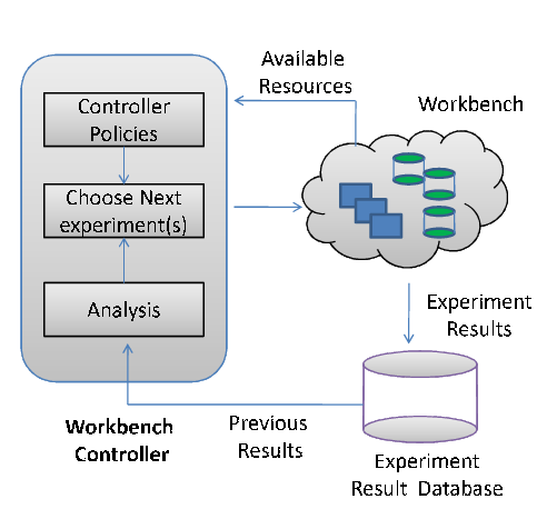
This paper investigates workbench automation techniques for server benchmarking. The objective is to devise a framework for an automated workbench controller that can implement various policies to coordinate experiments on a shared hardware pool or "workbench", e.g., a virtualized server cluster with programmatic interfaces to allocate and configure server resources [12,27]. The controller plans a set of experiments according to some policy, obtains suitable resources at a suitable time for each experiment, configures the test harness (system under test and workload generators) on those resources, launches the experiment, and uses the results and workbench status as input to plan or adjust the next experiments, as depicted in Figure 1. Our goal is to choreograph a set of experiments to obtain a statistically sound result for a high-level objective at low cost, which may involve using different statistical thresholds to balance cost and accuracy for different runs in the set.

As a motivating example, this paper focuses on the problem of measuring the peak throughput attainable by a given server configuration under a given workload (the saturation throughput or peak rate). Even this relatively simple objective requires a costly set of experiments that have not been studied in a systematic way. This task is common in industry, e.g., to obtain a qualifying rating for a server product configuration using a standard server benchmark from SPEC, TPC, or some other body as a basis for competitive comparisons of peak throughput ratings in the marketplace. One example of a standard server benchmark is the SPEC SFS benchmark and its predecessors [15], which have been used for many years to establish NFSOPS ratings for network file servers and filer appliances using the NFS protocol.

Systems research often involves more comprehensive benchmarking activities. For example, response surface mapping plots system performance over a large space of workloads and/or system configurations. Response surface methodology is a powerful tool to evaluate design and cost tradeoffs, explore the interactions of workloads and system choices, and identify interesting points such as optima, crossover points, break-even points, or the bounds of the effective operating range for particular design choices or configurations [17]. Figure 2 gives an example of response surface mapping using the peak rate. The example is discussed in Section 2. Measuring a peak rate is the "inner loop" for this response surface mapping task and others like it.

This paper illustrates the power of a workbench automation framework by exploring simple policies to optimize the "inner loop" to obtain peak rates in an efficient way. We use benchmarking of Linux-based NFS servers with a configurable workload generator as a running example. The policies balance cost, accuracy, and confidence for the result of each test load, while meeting target levels of confidence and accuracy to ensure statistically rigorous final results. We also show how advanced controllers can implement heuristics for efficient response surface mapping in a multi-dimensional space of workloads and configuration settings.

2 Overview

**Figure 1:** Automated Workbench and Controller.
$\begin{figure}\centering \epsfig{file=graphs/controller2,width=7cm,bbllx=174,bbl... ...rx=544,bbury=705,angle =270,clip=true} \vspace{-2ex}\vspace{-2ex} \end{figure}$

Figure 1 depicts a framework for automated server benchmarking. An automated workbench controller directs benchmarking experiments on a common hardware pool (workbench). The controller incorporates policies that decide which experiments to conduct and in what order, based on the following considerations:

**Figure 2:** These surfaces illustrate how the peak rate, $\lambda ^*$ , changes with number of disks and number of NFS daemon (nfsd) threads for two canned *fstress* workloads (**DB_TP** and **Web server**) on Linux-based NFS servers. The workloads for this example are described in more detail later, in Table 3.
$\begin{figure}\centering \epsfig{file=graphs/surface_database.eps,width=8cm} \e... ...aphs/surface_webserver.eps,width=8cm} \vspace{-2ex}\vspace{-2ex} \end{figure}$

Table 1: Some workload and configuration factors that affect NFS file server performance.

$\vec{W}$	read/write ratio, random/sequential ratio, metadata/data ratio, dataset size, file size distribution, directory structure, request mix
$\vec{R}$	CPU speed, memory size, number of disks
$\vec{C}$	Number of NFS server I/O daemons (nfsds), type of file system, block size

We characterize the benchmark performance of a server by its peak rate or saturation throughput, denoted $\lambda ^*$ . $\lambda ^*$ is the highest request arrival rate $\lambda$ that does not drive the server into a saturation state. The server is said to be in a saturation state if a response time metric exceeds a specified threshold, indicating that the offered load has reached the maximum that the server can process effectively.

The performance of a server is a function of its workload, its configuration, and the hardware resources allocated to it. Each of these may be characterized by a vector of metrics or factors, as summarized in Table 1.

Workload $\vec{W}$ . Workload factors define the properties of the request mix and the data sets they operate on, and other workload characteristics.

Configurations ( $\vec{C}$ ). The controller may vary server configuration parameters (e.g., buffer sizes, queue bounds, concurrency levels) before it instantiates the server for each run.

Resources $\vec{R}$ . The controller can vary the amount of hardware resources assigned to the system under test, depending on the capabilities of the workbench testbed. The prototype can instantiate Xen virtual machines sized along the memory, CPU, and I/O dimensions. The experiments in this paper vary the workload and configuration parameters on a fixed set of Linux server configurations in the workbench.

2.1 Example: NFS Server Benchmarking

This paper uses NFS server benchmarking as a running example. The controllers use a configurable synthetic NFS workload generator called Fstress [1], which was developed in previous research. Fstress offers knobs for various workload factors ( $\vec{W}$ ), enabling the controller to configure the properties of the workload's dataset and its request mix to explore a space of NFS workloads. Fstress has preconfigured parameter sets that represent standard NFS file server workloads (e.g., SPECsfs97, Postmark), as well as many other workloads that might be encountered in practice (see Table 3).

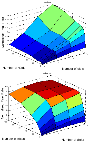
Figure 2 shows an example of response surfaces produced by the automated workbench for two canned NFS server workloads representing typical request mixes for a file server that backs a database server (called DB_TP) and a static Web server (Web server). A response surface gives the response of a metric (peak rate) to changes in the operating range of combinations of factors in a system [17]. In this illustrative example the factors are the number of NFS server daemons (nfsds) and disk spindle counts.

Response surface mapping can yield insights into the performance effects of configuration choices in various settings. For example, Figure 2 confirms the intuition that adding more disks to an NFS server can improve the peak rate only if there is a sufficient number of nfsds to issue requests to those disks. More importantly, it also reveals that the ideal number of nfsds is workload-dependent: standard rules of thumb used in the field are not suitable for all workloads.

2.2 Problem Statement

The challenge for the automated feedback-driven workbench controller is to design a set of experiments to obtain accurate peak rates for a set of test points, and in particular for test points selected to approximate a response surface efficiently.

Response surface mapping is expensive. Algorithm 1 presents the overall benchmarking approach that is used by the workbench controller to map a response surface, and Table 2 summarizes some relevant notation. The overall approach consists of an outer loop that iterates over selected samples from $\langle F_1, \ldots, F_n \rangle$ , where $F_1, \ldots, F_n$ is a subset of factors in the larger $\langle \vec{W}, \vec{R}, \vec{C}\rangle$ space (Step 2). The inner loop (Step 3) finds the peak rate $\lambda ^*$ for each sample by generating a series of test loads for the sample. For each test load $\lambda$ , the controller must choose the runlength

or observation interval, and the number of independent trials

to obtain a response time measure under load $\lambda$ .

The goal of the automated feedback-driven controller is to address the following problems.

Minimizing benchmarking cost involves choosing values carefully for the runlength

, the number of trials

, and test loads $\lambda$ so that the controller converges quickly to the peak rate. Sections 3 and 4 present algorithms that the controller uses to address these problems.

2.3 Confidence and Accuracy

Benchmarking can never produce an exact result because complex systems exhibit inherent variability in their behavior. The best we can do is to make a probabilistic claim about the interval in which the "true" value for a metric lies based on measurements from multiple independent trials [13]. Such a claim can be characterized by a confidence level and the confidence interval at this confidence level. For example, by observing the mean response time $\bar{R}$ at a test load $\lambda$ for

independent trials, we may be able to claim that we are

% confident (the confidence level) that the correct value of $\bar{R}$ for that $\lambda$ lies within the range

(the confidence interval).

Basic statistics tells us how to compute confidence intervals and levels from a set of trials. For example, if the mean server response time $\bar{R}$ from

trials is $\mu$ , and standard deviation is $\sigma$ , then the confidence interval for $\mu$ at confidence level

is given by:

is a reading from the table of standard normal distribution for confidence level

. If

, then we use Student's t distribution instead after verifying that the

runs come from a normal distribution [13].

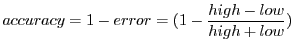
The tightness of the confidence interval captures the accuracy of the true value of the metric. A tighter bound implies that the mean response time from a set of trials is closer to its true value. For a confidence interval

, we compute the percentage accuracy as:

Table 2: Benchmarking parameters used in this paper.

$\lambda ^*$	Peak rate for a given server configuration and workload.
$\lambda$	Offered load (arrival rate) for a given test load level.
$\rho$	Load factor $=\lambda/\lambda^*$ for a test load $\lambda$ .
$\bar{R}$	Mean server response time for a test load.
$R_{sat}$	Threshold for $\bar{R}$ at the peak rate: the server is saturated if $\bar{R} > R_{sat}$ .
	Factor that determines the width of the peak-rate region $[R_{sat} \pm sR_{sat}]$ (§3.3).
	Target accuracy (based on confidence interval width) for the estimated value of $\lambda ^*$ (§2.3).
	Target confidence level for the estimated $\lambda ^*$ (§2.3).
	Number of independent trials at a test load.
	Runlength: the test interval over which to observe the server latency for each trial.

$\begin{algorithm} % latex2html id marker 275 [t] \caption{Mapping Response Surfa... ...he server to the saturation state\; } \end{list} \vspace{-3ex} \end{algorithm}$

3 Finding the Peak Rate

In the inner loop of Algorithm 1, the automated controller searches for the peak rate $\lambda ^*$ for some workload and configuration given by a selected sample of factor values in $\langle F_1, \ldots, F_n \rangle$ . To find the peak rate it subjects the server to a sequence of test loads $\lambda = [\lambda_1, \ldots, \lambda_l]$ . The sequence of test loads should converge on an estimate of the peak rate $\lambda ^*$ that meets the target accuracy and confidence.

We emphasize that this step is itself a common benchmarking task to determine a standard rating for a server configuration in industry (e.g., SPECsfs [6]).

3.1 Strawman: Linear Search with Fixed

and

Common practice for finding the peak rate is to script a sequence of runs for a standard workload at a fixed linear sequence of escalating load levels, with a preconfigured runlength

and number of trials

for each load level. The algorithm is in essence a linear search for the peak rate: it starts at a default load level and increments the load level (e.g., arrival rate) by some fixed increment until it drives the server into saturation. The last load level $\lambda$ before saturation is taken as the peak rate $\lambda ^*$ . We refer to this algorithm as strawman.

**Figure 3:** An efficient policy for finding peak rate converges quickly to a load factor near , and reduces benchmarking cost by obtaining a high-confidence result only for the load factor of . It is significantly less costly than the *strawman* policy: a linear search with a fixed runlength and fixed number of trials per test load.
$\begin{figure}\centering \epsfig{file=graphs/cartoon_time_loadfactor_1.eps, width=8cm} \vspace{-4ex}\vspace{-2ex} \end{figure}$

**Figure 4:** Mean server response time at different test loads for the **DB_TP** fstress workload using disk and NFS daemon (nfsd) threads for the server. The variability in mean server response time for multiple trials increases with load. The results are representative of other server configurations and workloads.
$\begin{figure}\centering \epsfig{file=graphs/shivam_physical_shivam10_diagnostic... ...ressload.response_load.eps, width=8cm} \vspace{-4ex}\vspace{-2ex} \end{figure}$

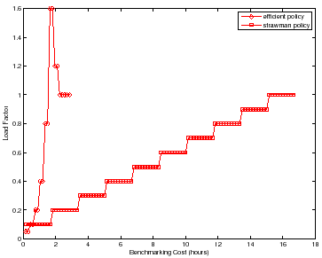
Strawman is not efficient. If the increment is too small, then it requires many iterations to reach the peak rate. Its cost is also sensitive to the difference between the peak rate and the initial load level: more powerful server configurations take longer to benchmark. A larger increment can converge on the peak rate faster, but then the test may overshoot the peak rate and compromise accuracy. In addition, strawman misses opportunities to reduce cost by taking "rough" readings at low cost early in the search, and to incur only as much cost as necessary to obtain a statistically sound reading once the peak rate is found.

A simple workbench controller with feedback can improve significantly on the strawman approach to searching for the peak rate. To illustrate, Figure 3 depicts the search for $\lambda ^*$ for two policies conducting a sequence of experiments, with no concurrent testing. For strawman we use runlength

minutes,

trials, and a small increment to produce an accurate result. The figure compares strawman to an alternative that converges quickly on the peak rate using binary search, and that adapts

and

dynamically to balance accuracy, confidence, and cost during the search. The figure represents the sequence of actions taken by each policy with cumulative benchmarking time on the x-axis; the y-axis gives the load factor $\rho = \frac{\lambda}{\lambda^*}$ for each test load evaluated by the policies. The figure shows that strawman can incur a much higher benchmarking cost (time) to converge to the peak rate and complete the search with a final accurate reading at load factor $\rho = 1$ . The strawman policy not only evaluates a large number of test loads with load factors that are not close to

, but also incurs unnecessary cost at each load.

The remainder of the paper discusses the improved controller policies in more detail, and their interactions with the outer loop in mapping response surfaces.

3.2 Choosing

and

for Each Test Load

The runlength

and the number of trials

together determine the benchmarking cost incurred at a given test load $\lambda$ . The controller should choose

and

to obtain the confidence and accuracy desired for each test load at least cost. The goal is to converge quickly to an accurate reading at the peak rate: $\lambda = \lambda^*$ and load factor $\rho = 1$ . High confidence and accuracy are needed for the final test load at $\lambda = \lambda^*$ , but accuracy is less crucial during the search for the peak rate. Thus the controller has an opportunity to reduce benchmarking cost by adapting the target confidence and accuracy for each test load $\lambda$ as the search progresses, and choosing

and

for each $\lambda$ appropriately.

At any given load level the controller can trade off confidence and accuracy for lower cost by decreasing either

or both. Also, at a given cost any given set of trials and runlengths can give a high-confidence result with wide confidence intervals (low accuracy), or a narrower confidence interval (higher accuracy) with lower confidence.

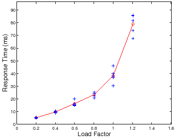
However, there is a complication: performance variability tends to increase as the load factor $\rho$ approaches saturation. Figure 4 and Figure 5 illustrate this effect. Figure 4 is a scatter plot of mean server response time ( $\bar{R}$ ) at different test loads $\lambda$ for five trials at each load. Note that the variability across multiple trials increases as $\lambda \rightarrow \lambda^*$ and $\rho \rightarrow 1$ . Figure 5 shows a scatter plot of $\bar{R}$ measures for multiple runlengths at two load factors, $\rho = 0.3$ and $\rho = 0.9$ . Longer runlengths show less variability at any load factor, but for a given runlength, the variability is higher at the higher load factor. Thus the cost for any level of confidence and/or accuracy also depends on load level: since variability increases at higher load factors, it requires longer runlengths

and/or a larger number of trials

to reach a target level of confidence and accuracy.

For example, consider the set of trials plotted in Figure 5. At load factor

and runlength of

seconds, the data gives us

% confidence that $5.6 < \bar{R} < 6$ , or

% confidence that $5 < \bar{R} < 6.5$ . From the data we can determine the runlength needed to achieve target confidence and accuracy at this load level and number of trials

: a runlength of

seconds achieves an accuracy of

% with

% confidence, but it takes a runlength of

seconds to achieve

% accuracy with

% confidence. Accuracy and confidence decrease with higher load factors. For example, at load factor

and runlength

, the data gives us

% confidence that $21 < \bar{R} < 24$ (

% accuracy), or

% confidence that $20 < \bar{R} < 27$ (

% accuracy). As a result, we must increase the runlength and/or the number of trials to maintain target levels of confidence and accuracy as load factors increase. For example, we need a runlength of

seconds or more to achieve accuracy $\geq 87$ % at

% confidence for this number of trials at load factor

Figure 6 quantifies the tradeoff between the runlength and the number of trials required to attain a target accuracy and confidence for different workloads and load factors. It shows the number of trials required to meet an accuracy of

% at

% confidence level for different runlengths. The figure shows that to attain a target accuracy and confidence, one needs to conduct more independent trials at shorter runlengths. It also shows a sweet spot for the runlengths that reduces the number of trials needed. A controller can use such curves as a guide to pick a suitable runlength

and number of trials

with low cost.

**Figure 5:** Mean server response time $\bar{R}$ at different workload runlengths for the **DB_TP** fstress workload using disk and NFS daemon (nfsd) threads for the server. The variability in mean server response time for multiple trials decreases with increase in runlength. The results are representative of other server configurations and workloads.
$\begin{figure}\centering \epsfig{file=graphs/shivam_physical_shivam9_diagnostic... ....response_runtime_200.eps, width=8cm} \vspace{-2ex}\vspace{-2ex} \end{figure}$

**Figure 6:** Number of trials to attain % accuracy for mean server response time at % confidence level at low and high load factors for different runlengths. The results are for server configuration with disk and nfsds, and representative of other server configurations.
$\begin{figure}\centering \epsfig{file=graphs/multi_workloads_numruns_runtime_tr... ...runtime_tradeoff_high.eps, width=8cm} \vspace{-2ex}\vspace{-2ex} \end{figure}$

3.3 Search Algorithm

Our approach uses Algorithm 2 to search for the peak rate for a given setting of factors.

Algorithm 2 takes various parameters to define the conditions for the reported peak rate:

Algorithm 2 chooses (a) a sequence of test loads to try; (b) the number of independent trials at any test load; and (c) the runlength of the workload at that load. It automatically adapts the number of trials at any test load according to the load factor and the desired target confidence and accuracy. At each load level the algorithm conducts a small (often the minimum of two in our experiments) number of trials to establish with

% confidence that the current test load is not the peak rate (Step

). However, as soon as the algorithm identifies a test load $\lambda$ to be a potential peak rate, which happens near a load factor of

, it spends just enough time to check whether it is in fact the peak rate.

More specifically, for each test load $\lambda _{cur}$ , Algorithm 2 first conducts two trials to generate an initial confidence interval for $\bar{R}_{\lambda_{cur}}$ , the mean server response time at load $\lambda _{cur}$ , at

% confidence level. (Steps

and

in Algorithm 2.) Next, it checks if the confidence interval overlaps with the specified peak-rate region (Step

If the regions overlap, then Algorithm 2 identifies the current test load $\lambda _{cur}$ as an estimate of a potential peak rate with 95% confidence. It then computes the accuracy of the mean server response time $\bar{R}_{\lambda_{cur}}$ at the current test load, at the target confidence level

(Section 2.1). If it reaches the target accuracy

, then the algorithm terminates (Step

), otherwise it conducts more trials at the current test load (Step

) to narrow the confidence interval, and repeats the threshold condition test. Thus the cost of the algorithm varies with the target confidence and accuracy.

If there is no overlap (Step

), then Algorithm 2 moves on to the next test load. It uses any of several load-picking algorithms to generate the sequence of test loads, described in the rest of this section. All load-picking algorithms take as input the set of past test loads and their results. The output becomes the next test load in Algorithm 2. For example, Algorithm 3 gives a load-picking algorithm using a simple binary search.

To simplify the choice of runlength for each experiment at a test load (Step 5), Algorithm 2 uses the "sweet spot" derived from Figure 6 (Section 3.2). The figure shows that for all workloads that this paper considers, a runlength of

minutes is the sweet spot for the minimum number of trials.

3.4 The Binsearch Load-Picking Algorithm

Algorithm 3 outlines the Binsearch algorithm. Intuitively, Binsearch keeps doubling the current test load until it finds a load that saturates the server. After that, Binsearch applies regular binary search, i.e., it recursively halves the most recent interval of test loads where the algorithm estimates the peak rate to lie.

Binsearch allows the controller to find the lower and upper bounds for the peak rate within a logarithmic number of test loads. The controller can then estimate the peak rate using another logarithmic number of test loads. Hence the total number of test loads is always logarithmic irrespective of the start test load or the peak rate.

$\begin{algorithm} % latex2html id marker 1051 [t] \caption{Binsearch {\bf Input}... ...earch$_{low}$)/$2$\; \vspace{-1ex} \par \end{list}\vspace{-2ex} \end{algorithm}$

3.5 The Linear Load-Picking Algorithm

The Linear algorithm is similar to Binsearch except in the initial phase of finding the lower and upper bounds for the peak rate. In the initial phase it picks an increasing sequence of test loads such that each load differs from the previous one by a small fixed increment.

3.6 Model-guided Load-Picking Algorithm

The general shape of the response-time vs. load curve is well known, and the form is similar for different workloads and server configurations. This suggests that a model-guided approach could fit the curve from a few test loads and converge more quickly to the peak rate. Using the insight offered by well-known open-loop queuing theory results [13], we experimented with a simple model to fit the curve: $R = 1/(a - b*\lambda)$ , where

is the response time, $\lambda$ is the load, and

and

are constants that depend on the settings of factors in $\langle \vec{W}, \vec{R}, \vec{C}\rangle$ . To learn the model, the controller needs tuples of the form $\langle \lambda, R_{\lambda} \rangle$ .

Algorithm 4 outlines the model-guided algorithm. If there are insufficient tuples for learning the model, it uses a simple heuristic to pick the test loads for generating the tuples. After that, the algorithm uses the model to predict the peak rate $\lambda = \lambda^*$ for $R = R_{sat}$ , returns the prediction as the next test load, and relearns the model using the new $\langle \lambda, R_{\lambda} \rangle$ tuple at the prediction. The whole process repeats until the search converges to the peak rate. As the controller observes more $\langle \lambda, R_{\lambda} \rangle$ tuples, the model-fit should improve progressively, and the model should guide the search to an accurate peak rate. In many cases, this happens in a single iteration of model learning (Section 5).

However, unlike the previous approaches, a model-guided search is not guaranteed to converge. Model-guided search is dependent on the accuracy of the model, which in turn depends on the choice of $\langle \lambda, R_{\lambda} \rangle$ tuples that are used for learning. The choice of tuples is generated by previous model predictions. This creates the possibility of learning an incorrect model which in turn yields incorrect choices for test loads. For example, if most of the test loads chosen for learning the model happen to lie significantly outside the peak rate region, then the model-guided choice of test loads may be incorrect or inefficient. Hence, in the worst case, the search may never converge or converge slowly to the peak rate. We have experimented with other models including polynomial models of the form $R=a + b\lambda + c\lambda^2$ , which show similar limitations.

To avoid the worst case, the algorithm uses a simple heuristic to choose the tuples from the list of available tuples. Each time the controller learns the model, it chooses two tuples such that one of them is the last prediction, and the other is the tuple that yields the response time closest to threshold mean server response time $R_{sat}$ . More robust techniques for choosing the tuples is a topic of ongoing study. Section 5 reports our experience with the model-guided choice of test loads. Preliminary results suggest that the model-guided approaches are often superior but can be unstable depending on the initial samples used to learn the model.

$\begin{algorithm} % latex2html id marker 1514 [t] \caption{Model-Guided {\bf Inp... ...a,b$ are the fitted coefficients\; \par \end{list}\vspace{-3ex} \end{algorithm}$

3.7 Seeding Heuristics

The load-picking algorithms in Sections 3.5-3.6 generate a new load given one or more previous test loads. How can the controller generate the first load, or seed, to try? One way is to use a conservative low load as the seed, but this approach increases the time spent ramping up to a high peak rate. When the benchmarking goal is to plot a response surface, the controller uses another approach that uses the peak rate of the "nearest" previous sample as the seed.

To illustrate, assume that the factors of interest, $\langle F_1, \ldots, F_n \rangle$ , in Algorithm 1 are $\langle$ number of disks, number of nfsds $\rangle$ (as shown in Figure 2). Suppose the controller uses Binsearch with a low seed of

to find the peak rate $\lambda^{*}_{1,1}$ for sample $\langle 1, 1 \rangle$ . Now, for finding the peak rate $\lambda^{*}_{1,2}$ for sample $\langle 1, 2 \rangle$ , it can use the peak rate $\lambda^*_{1,1}$ as seed. Thus, the controller can jump quickly to a load value close to $\lambda^{*}_{1,2}$ .

In the common case, the peak rates for "nearby" samples will be close. If they are not, the load-picking algorithms may incur additional cost to recover from a bad seed. The notion of "nearnest" is not always well defined. While the distance between samples can be measured if the factors are all quantitative, if there are categorical factors--e.g., file system type--the nearest sample may not be well defined. In such cases the controller may use a default seed or an aggregate of peak rates from previous samples to start the search.

4 Mapping Response Surfaces

We now relate the peak rate algorithm that Section 3 describes to the larger challenge of mapping a peak rate response surface efficiently and effectively, based on Algorithm 1.

A large number of factors can affect performance, so it is important to sample the multi-dimensional space with care as well as to optimize the inner loop. For example, suppose we are mapping the impact of five factors on a file server's peak rate, and that we sample five values for each factor. If the benchmarking process takes an hour to find the peak rate for each factor combination, then the total time for benchmarking is

days. An automated workbench controller can shorten this time by pruning the sample space, planning experiments to run on multiple hardware setups in parallel, and optimizing the inner loop.

If the benchmarking objective is to understand the overall trend of how the peak rate is affected by certain factors of interest $\langle F_1, \ldots, F_n \rangle$ --rather than finding accurate peak rate values for each sample in $\langle F_1, \ldots, F_n \rangle$ --then Algorithm 1 can leverage Response Surface Methodology (RSM) [17] to select the sample points efficiently (in Step 2). RSM is a branch of statistics that provides principled techniques to choose a set of samples to obtain good approximations of the overall response surface at low cost. For example, some RSM techniques assume that a low-degree multivariate polynomial model-- e.g., a quadratic equation of the form $\lambda^* = \beta_0 + \sum_{i=1}^n \beta_{i} F_i + \sum_{i=1}^n \sum_{j=1, j \neq i}^n \beta_{ij} F_iF_j + \sum_{i=1}^n \beta_{ii} {F_i}^2$ -- approximates the surface in the

-dimensional $\langle F_1, \ldots, F_n \rangle$ space. This approximation is a basis for selecting a minimal set of samples for the controller to obtain in order to learn a fairly accurate model (i.e., estimate values of the $\beta$ parameters in the model). We evaluate one such RSM technique in Section 5.

It is important to note that these RSM techniques may reduce the effectiveness of the seeding heuristics described in Section 3.7. RSM techniques try to find sample points on the surface that will add the most information to the model. Intuitively, such samples are the ones that we have the least prior information about, and hence for which seeding from prior results would be least effective. We leave it to future work to explore the interactions of the heuristics for selecting samples efficiently and seeding the peak rate search for each sample.

5 Experimental Evaluation

Cost for Finding Peak Rate. Sections 3.3 and 4 present several policies for finding the peak rate. We evaluate those policies as follows:

Cost for Mapping Response Surfaces. We compare the total benchmarking cost for mapping the response surface across all the samples.

Cost Versus Target Confidence and Accuracy. We demonstrate that the policies adapt the total benchmarking cost to target confidence and accuracy. Higher confidence and accuracy incurs higher benchmarking cost and vice-versa.

Section 5.1 presents the experiment setup. Section 5.2 presents the workloads that we use for evaluation. Section 5.3 evaluates our benchmarking methodology as described above.

5.1 Experimental Setup

Table 1 shows the factors in the $\langle \vec{W}, \vec{R}, \vec{C}\rangle$ vectors for a storage server. We benchmark an NFS server to evaluate our methodology. In our evaluation, the factors in $\vec{W}$ consist of samples that yield four types of workloads: SPECsfs97, Web server, Mail server, and DB_TP (Section 5.2). The controller uses Fstress to generate samples of $\vec{W}$ that correspond to these workloads. We report results for a single factor in $\vec{R}$ : the number of disks attached to the NFS server in $\langle 1, 2, 3, 4 \rangle$ , and a single factor in $\vec{C}$ : the number of nfsd daemons for the NFS server chosen from $\langle 1,2,4,8,16,32,64,100 \rangle$ to give us a total of

samples.

The workbench tools can generate both virtual and physical machine configurations automatically. In our evaluation we use physical machines that have

MB memory,

GHz x86 CPU, and run the

Linux kernel. To conduct an experiment, the workbench controller first prepares an experiment by generating a sample in $\langle \vec{W}, \vec{R}, \vec{C}\rangle$ . It then consults the benchmarking policy(ies) in Sections 3.4-4 to plot a response surface and/or search for the peak rate for a given sample with target confidence and accuracy.

5.2 Workloads

Table 3: Summary of fstress workloads used in the experiments.

workload	file popularities	file sizes	dir sizes	I/O accesses
SPECsfs97	random 10%	1 KB - 1 MB	large (thousands)	random r/w
Web server	Zipf ( $0.6<\alpha<0.9$ )	long-tail (avg 10.5 KB)	small (dozens)	sequential reads
DB_TP	few files	large (GB - TB)	small	random r/w
Mail	Zipf ( $\alpha = 1.3$ )	long-tail (avg 4.7 KB)	large (500+)	seq r, append w

We use Fstress to generate $\vec{W}$ corresponding to four workloads as summarized in Table 3. A brief summary follows. Further details are in [1].

5.3 Results

For evaluating the overall methodology and the policies outlined in Sections 3.3 and 4, we define the peak rate $\lambda ^*$ to be the test load that causes: (a) the mean server response time to be in the

ms region; or (b) the 95-percentile request response time to exceed

ms to complete. We derive the

region by choosing mean server response time threshold at the peak rate $R_{sat}$ to be

ms and the width factor $s = 10\%$ in Table 2. For all results except where we note explicitly, we aim for a $\lambda ^*$ to be accurate within

% of its true value with

% confidence.

5.3.1 Cost for Finding Peak Rate

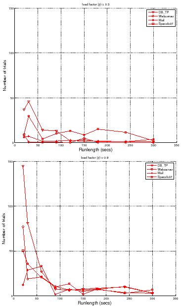
Figure 7 shows the choice of load factors for finding the peak rate for a sample with

disks and

nfsds using the policies outlined in Section 4. Each point on the curve represents a single trial for some load factor. More points indicate higher number of trials at that load factor. For brevity, we show the results only for DB_TP. Other workloads show similar behavior.

For all policies, the controller conducts more trials at load factors near

than at other load factors to find the peak rate with the target accuracy and confidence. All policies without seeding start at a low load factor and take longer to reach a load factor of

as compared to policies with seeding. All policies with seeding start at a load factor close to

, since they use the peak rate of a previous sample with

disks and

nfsds as the seed load.

Linear takes a significantly longer time because it uses a fixed increment by which to increase the test load. However, Binsearch jumps to the peak rate region in logarithmic number of steps. The Model policy is the quickest to jump near the load factor of

, but incurs most of its cost there. This happens because the model learned is sufficiently accurate for guiding the search near the peak rate, but not accurate enough to search the peak rate quickly.

**Figure 7:** Time spent at each load factor for finding the peak rate for different policies for **DB_TP** with disks and nfsds. Seeded policies were seeded with the peak rate for disks and nfsds. The result is representative of other samples and workloads. All policies except linear quickly converge to the load factor of and conduct more trials there to achieve the target accuracy and confidence.
$\begin{figure}\centering \epsfig{file=graphs/multi_workloads_time_loadfactor_3_database.eps, width=8cm} \vspace{-4ex}\vspace{-2ex} \end{figure}$

5.3.2 Cost for Mapping Response Surfaces

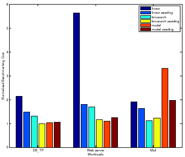
We also observe that Binsearch, Binsearch with Seeding, and Linear with Seeding are robust across the workloads, but the model-guided policy is unstable. This is not surprising given that the accuracy of the learned model guides the search. As Section 3.6 explains, if the model is inaccurate the search may converge slowly.

The linear policy is inefficient and highly sensitive to the magnitude of peak rate. The benchmarking cost of Linear for Web server peaks at a higher absolute value for all samples than for DB_TP and Mail, causing more than a factor of

increase in the total cost for mapping the surface. Note that for Mail, Binsearch with Seeding incurs a slightly higher cost than Binsearch. For some configurations, as Section 3.7 explains, seeding can incur additional cost to recover from a bad seed resulting in longer search times.

**Figure 8:** The total cost for mapping response surfaces for three workloads using different policies.
$\begin{figure}\centering \epsfig{file=graphs/total_time.eps, width=8cm} \vspace{-5ex}\vspace{-2ex} \end{figure}$

Reducing the Number of Samples. To evaluate the RSM approach presented in Section 4, we approximate the response surface by a quadratic curve in two dimensions: peak rate = func(number of disks, number of nfsds). We use a D-optimal design [17] from RSM to obtain the best of

and

samples out of a total of

samples for learning the response surface equation. We use Binsearch to obtain the peak rate for each.

After learning the equation, we use it to predict the peak rate at all the other samples in the surface. Table 4 presents the mean absolute percentage error in predicting the peak rate across all the samples. The results show that D-optimal designs do a very good job of picking appropriate samples, and that very little more can be learned by small increases in the number of points sampled. Improving the accuracy of the surface with limited numbers of sampled points is an area of ongoing research.

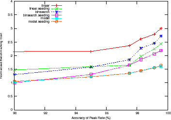
5.3.3 Cost Versus Target Confidence and Accuracy

Figure 9 shows how the benchmarking methodology adapts the total benchmarking cost to the target confidence and accuracy of the peak rate. The figure shows the total benchmarking cost for mapping the response surface for the DB_TP using the Binsearch policy for different target confidence and accuracy values.

Higher target confidence and accuracy incurs higher benchmarking cost. At

% accuracy, note the cost difference between the different confidence levels. Other workloads and policies exhibit similar behavior, with Mail incurring a normalized benchmarking cost of

at target accuracy of

% and target confidence of

**Figure 9:** The total benchmarking cost adapts to the desired confidence and accuracy. The cost is shown for mapping the response surface for **DB_TP** using the Binsearch policy. Other workloads and policies show similar results.
$\begin{figure}\centering \epsfig{file=graphs/time_accuracy_tradeoff_database.eps, width=8cm} \vspace{-4ex}\vspace{-2ex} \end{figure}$

So far, we configure the target accuracy of the peak rate by configuring the accuracy,

, of the response time at the peak rate. The width parameter

also controls the accuracy of the peak rate (Table 2) by defining the peak rate region. For example,

% implies that if the mean server response time at a test load is within

% of the threshold mean server response time, $R_{sat}$ , then the controller has found the peak rate. As the region narrows, the target accuracy of the peak rate region increases. In our experiments so far, we fix

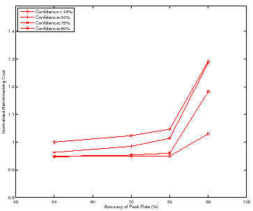
Figure 10 shows the benchmarking cost adapting to the target accuracy of the peak rate region for different policies at a fixed target confidence interval for DB_TP (

) and fixed target accuracy of the mean server response time at the peak rate (

%). The results for other workloads are similar. All policies except the model-guided policy incur the same benchmarking cost near or at the peak rate since all of them do binary search around that region. Since a narrower peak rate region causes more trials at or near load factor of

, the cost for these policies converge.

**Figure 10:** Benchmarking cost adapts to the target accuracy of the peak rate region for all policies. As the region narrows, the majority of the cost is incurred at or near the peak rate. Linear and Binsearch incur the same cost close to the peak rate, and hence their cost converges as they conduct more trials near the peak rate. The cost is shown for **DB_TP**. Other workloads show similar results.
$\begin{figure}\centering \epsfig{file=graphs/width.database.eps, width=8cm} \vspace{-4ex}\vspace{-2ex} \end{figure}$

6 Related Work

Several researchers have made a case for statistically significant results from system benchmarking, e.g., [4]. Auto-pilot [26] is a system for automating the benchmarking process: it supports various benchmark-related tasks and can modulate individual experiments to obtain a target confidence and accuracy. Our goal is to take the next step and focus on an automation framework and policies to orchestrate sets of experiments for a higher level benchmarking objective, such as evaluating a response surface or obtaining saturation throughputs under various conditions. We take the workbench test harness itself as given, and our approach is compatible with advanced test harnesses such as Auto-pilot.

While there are large numbers and types of benchmarks, (e.g., [5,14,3,15]) that test the performance of servers in a variety of ways, there is a lack of a general benchmarking methodology that provides benchmarking results from these benchmarks efficiently with confidence and accuracy. Our methodology and techniques for balancing the benchmarking cost and accuracy are applicable to all these benchmarks.

Zadok et al. [25] present an exhaustive nine-year study of file system and storage benchmarking that includes benchmark comparisons, their pros and cons [22], and makes recommendations for systematic benchmarking methodology that considers a range of workloads for benchmarking the server. Smith et al. [23] make a case for benchmarks the capture composable elements of realistic application behavior. Ellard et al. [10] show that benchmarking an NFS server is challenging because of the interactions between the server software configurations, workloads, and the resources allocated to the server. One of the challenges in understanding the interactions is the large space of factors that govern such interactions. Our benchmarking methodology benchmarks a server across the multi-dimensional space of workload, resource, and configuration factors efficiently and accurately, and avoids brittle "claims" [16] and "lies" [24] about a server performance.

Synthetic workloads emulate characteristics observed in real environments. They are often self-scaling [5], augmenting their capacity requirements with increasing load levels. The synthetic nature of these workloads enables them to preserve workload features as the file set size grows. In particular, the SPECsfs97 benchmark [6] (and its predecessor LADDIS [15]) creates a set of files and applies a pre-defined mix of NFS operations. The experiments in this paper use Fstress [1], a synthetic, flexible, self-scaling NFS workload generator that can emulate a range of NFS workloads, including SPECsfs97. Like SPECsfs97, Fstress uses probabilistic distributions to govern workload mix and access characteristics. Fstress adds file popularities, directory tree size and shape, and other controls. Fstress includes several important workload configurations, such as Web server file accesses, to simplify file system performance evaluation under different workloads [23] while at the same time allowing standardized comparisons across studies.

Server benchmarking isolates the performance effects of choices in server design and configuration, since it subjects the server to a steady offered load independent of its response time. Relative to other methodologies such as application benchmarking, it reliably stresses the system under test to its saturation point where interesting performance behaviors may appear. In the storage arena, NFS server benchmarking is a powerful tool for investigation at all layers of the storage stack. A workload mix can be selected to stress any part of the system, e.g., the buffering/caching system, file system, or disk system. By varying the components alone or in combination, it is possible to focus on a particular component in the storage stack, or to explore the interaction of choices across the components.

7 Conclusion

This paper focuses on the problem of workbench automation for server benchmarking. We propose an automated benchmarking system that plans, configures, and executes benchmarking experiments on a common hardware pool. The activity is coordinated by an automated controller that can consider various factors in planning, sequencing, and conducting experiments. These factors include accuracy vs. cost tradeoffs, availability of hardware resources, deadlines, and the results reaped from previous experiments.

We present efficient and effective controller policies that plot the saturation throughput or peak rate over a space of workloads and system configurations. The overall approach consists of iterating over the space of workloads and configurations to find the peak rate for samples in the space. The policies find the peak rate efficiently while meeting target levels of confidence and accuracy to ensure statistically rigorous benchmarking results. The controller may use a variety of heuristics and methodologies to prune the sample space to map a complete response service, and this is a topic of ongoing study.

Cutting Corners: Workbench Automation
for Server Benchmarking