16th USENIX Security Symposium
Pp. 43–54 of the Proceedings
Language Identification of Encrypted VoIP Traffic:
Alejandra y Roberto or Alice and Bob?
Charles V. Wright, Lucas Ballard, Fabian Monrose, Gerald M. Masson,
{cvwright, lucas, fabian, masson}@jhu.edu
Department of Computer Science
Johns Hopkins University
Baltimore, MD, USA
Abstract
Voice over IP (VoIP) has become a popular protocol for making phone
calls over the Internet. Due to the potential transit of sensitive
conversations over untrusted network infrastructure, it is well
understood that the contents of a VoIP session should be encrypted.
However, we demonstrate that current cryptographic techniques do not
provide adequate protection when the underlying audio is encoded
using bandwidth-saving Variable Bit Rate (VBR) coders. Explicitly,
we use the length of encrypted VoIP packets to tackle the
challenging task of identifying the language of the conversation.
Our empirical analysis of 2,066 native speakers of 21 different
languages shows that a substantial amount of information can be
discerned from encrypted VoIP traffic. For instance, our 21-way
classifier achieves 66% accuracy, almost a 14-fold improvement over
random guessing. For 14 of the 21 languages, the accuracy is greater than 90%.
We achieve an overall binary classification (e.g., "Is this a
Spanish or English conversation?") rate of 86.6%. Our analysis
highlights what we believe to be interesting new privacy issues in VoIP.
1 Introduction
Over the last several years, Voice over IP (VoIP) has enjoyed a marked
increase in popularity, particularly as a replacement of traditional
telephony for international calls. At the same time, the security and
privacy implications of conducting everyday voice communications over
the Internet are not yet well understood. For the most part, the
current focus on VoIP security has centered around efficient
techniques for ensuring confidentiality of VoIP conversations
[3,
6,
14,
37].
Today, because of the success of these efforts and the attention they
have received, it is now widely accepted that VoIP traffic should be
encrypted before transmission over the Internet. Nevertheless, little,
if any, work has explored the threat of traffic analysis of encrypted
VoIP calls. In this paper, we show that although encryption prevents
an eavesdropper from reading packet contents and thereby listening in
on VoIP conversations (for example, using
[21]),
traffic analysis can still be used to infer more information than
expected-namely, the spoken language of the
conversation. Identifying the spoken language in VoIP communications
has several obvious applications, many of which have substantial
privacy ramifications
[7].
The type of traffic analysis we demonstrate in this paper is made
possible because current recommendations for
encrypting VoIP traffic (generally, the application of
length-preserving stream ciphers) do not conceal the size of the
plaintext messages. While leaking message size may not pose a
significant risk for more traditional forms of electronic
communication such as email, properties of real-time streaming media
like VoIP greatly increase the potential for an attacker to extract
meaningful information from plaintext length. For instance, the size
of an encoded audio frame may have much more meaningful semantics than
the size of a text document. Consequently, while the size of an email
message likely carries little information about its contents, the use
of bandwidth-saving techniques such as variable bit rate (VBR) coding
means that the size of a VoIP packet is directly determined by the
type of sound its payload encodes. This information leakage is
exacerbated in VoIP by the sheer number of packets that are sent,
often on the order of tens or hundreds every second. Access to such
large volumes of packets over a short period of time allows an
adversary to quickly estimate meaningful distributions over the packet
lengths, and in turn, to learn information about the language being
spoken.
Identifying spoken languages is a task that, on the surface, may seem simple.
However it is a problem that has not only received substantial attention in the
speech and natural language processing community, but has also been found to be
challenging even with access to full acoustic data. Our results show an
encrypted conversation over VoIP can leak information about its contents, to the
extent that an eavesdropper can successfully infer what language is being spoken.
The fact that VoIP packet lengths can be used to perform any sort of language
identification is interesting in and of itself. Our success with language
identification in this setting provides strong grounding for mandating the use
of fixed length compression techniques in VoIP, or for requiring the underlying
cryptographic engine to pad each packet to a common length.
The rest of this paper is organized as follows. We begin in Section
2 by reviewing why and how voice over IP technologies
leak information about the language spoken in an encrypted call. In Section
3, we describe our design for a classifier that
exploits this information leakage to automatically identify languages based on
packet sizes. We evaluate this classifier's effectiveness in Section
4, using open source VoIP software and audio
samples from a standard data set used in the speech processing community.
We review related work on VoIP security and information leakage attacks in
Section 5, and conclude in Section
6.
2 Information Leakage via Variable Bit Rate Encoding
To highlight why language identification is possible in encrypted VoIP streams,
we find it instructive to first review the relevant inner workings of a modern
VoIP system. Most VoIP calls use at least two protocols: (1) a signaling
protocol such as the Session Initiation Protocol (SIP)
[23] used for locating the callee and establishing
the call and (2) the Real Time Transport Protocol (RTP)
[25,4]
which transmits the audio data, encoded using a special-purpose speech codec, over
UDP. While several speech codecs are available (including G.711 [10], G.729 [12],
Speex [29], and iLBC
[2]), we choose the Speex codec for our
investigation as it offers several advanced features like a VBR mode and discontinuous
transmission, and its source code is freely available. Additionally, although Speex
is not the only codec to offer variable bit rate encoding for speech
[30,
16,
20,
35,
5],
it is the most popular of those that do.
Speex, like most other modern speech codecs, is based on
code-excited linear prediction (CELP) [24]. In CELP, the
encoder uses vector quantization with both a fixed codebook and an
adaptive codebook [22] to encode a window of n audio
samples as one frame. For example, in the Speex default narrowband
mode, the audio input is sampled at 8kHz, and the frames each encode
160 samples from the source waveform. Hence, a packet containing one
Speex frame is typically transmitted every 20ms. In VBR mode, the
encoder takes advantage of the fact that some sounds are easier to
represent than others. For example, with Speex, vowels and
high-energy transients require higher bit rates than fricative
sounds like "s" or "f" [28]. To achieve improved
sound quality and a low (average) bit rate, the encoder uses fewer
bits to encode frames which contain "easy" sounds and more bits
for frames with sounds that are harder to encode. Because the VBR
encoder selects the best bit rate for each frame, the size of a
packet can be used as a predictor of the bit rate used to encode the
corresponding frame. Therefore, given only packet lengths, it is
possible to extract information about the underlying speech. Figure
1, for example, shows an audio input, the encoder's
bit rate, and the resulting packet sizes as the information is sent
on the wire; notice how strikingly similar the last two cases are.
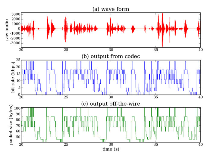 Figure 1: Uncompressed audio signal, Speex bit rates, and packet
sizes for a random sample from the corpus.
Figure 1: Uncompressed audio signal, Speex bit rates, and packet
sizes for a random sample from the corpus.
As discussed earlier, by now it is commonly accepted that VoIP traffic
should not be transmitted over the Internet without some additional
security layer [14,21]. Indeed, a number
of proposals for securing VoIP have already been introduced. One such
proposal calls for tunneling VoIP over IPSec, but doing so imposes
unacceptable delays on a real-time protocol [3]. An
alternative, endorsed by NIST [14],
is the Secure Real Time Transport Protocol (SRTP) [4]. SRTP is
an extension to RTP and provides confidentiality, authenticity, and
integrity for real-time applications. SRTP allows for three modes of
encryption: AES in counter mode, AES in f8-mode, and no encryption.
For the two stream ciphers, the standard states that "in case the
payload size is not an integer multiple of (the block length), the
excess bits of the key stream are simply discarded" [4].
Moreover, while the standard permits higher level protocols to pad
their messages, the default in SRTP is to use length-preserving
encryption and so one can still derive information about the
underlying speech by observing the lengths of the encrypted payloads.
Given that the sizes of encrypted payloads are closely related to bit
rates used by the speech encoder, a pertinent question is whether
different languages are encoded at different bit rates. Our
conjecture is that this is indeed the case, and to test this
hypothesis we examine real speech data from the Oregon Graduate
Institute Center for Speech Learning and Understanding's "22 Language"
telephone speech corpus [15].
The data set consists of speech from native speakers of 21
languages, recorded over a standard telephone line at 8kHz. This is
the same sampling rate used by the Speex narrowband mode.
General statistics about the data set are provided in
Appendix A.
As a preliminary test of our hypothesis, we encoded all of the audio
files from the CSLU corpus and recorded the sequence of bit rates used
by Speex for each file. In narrowband VBR mode with discontinuous
transmission enabled, Speex encodes the data set
using nine distinct bit rates, ranging from 0.25kbps up to 24.6kbps.
Figure 2 shows the frequency for each bit rate for
English, Brazilian Portuguese, German, and Hungarian. For most bit
rates, the frequencies for English are quite close to those for
Portuguese; but Portuguese and Hungarian appear to exhibit different
distributions. This results suggest that distinguishing Portuguese
from Hungarian, for example, would be less challenging than
differentiating Portuguese from English, or Indosesian from Russian
(see Figure 3).
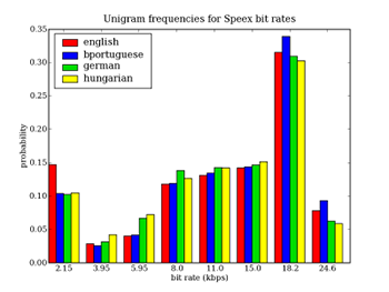 Figure 2: Unigram frequencies of bit rates for English, Brazilian
Portuguese, German and Hungarian
Figure 2: Unigram frequencies of bit rates for English, Brazilian
Portuguese, German and Hungarian
|
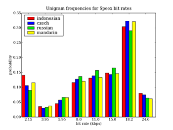 Figure 3: Unigram frequencies of bit rates for Indonesian,
Czech, Russian, and Mandarin
Figure 3: Unigram frequencies of bit rates for Indonesian,
Czech, Russian, and Mandarin
|
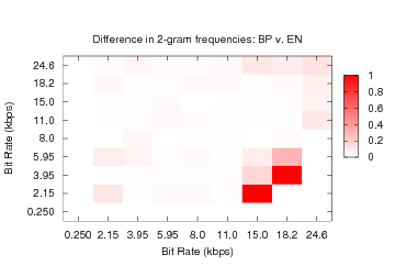 Figure 4: The normalized difference in bigram frequencies
between Brazilian Portuguese (BP) and English
(EN).
Figure 4: The normalized difference in bigram frequencies
between Brazilian Portuguese (BP) and English
(EN).
|
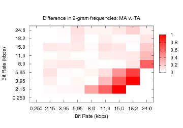 Figure 5: The normalized difference in bigram frequencies
between Mandarin (MA) and Tamil
(TA).
Figure 5: The normalized difference in bigram frequencies
between Mandarin (MA) and Tamil
(TA).
|
Figures 4 and 5
provide additional evidence that bigram frequencies (i.e., the number
of instances of consecutively observed bit rate pairs) differ between
languages. The x and y axes of both figures specify observed bit rates.
The density of the square (x,y) shows the difference in probability of
bigram x,y between the two languages divided by the average
probability of bigram x,y between the two. Thus, dark squares
indicate significant differences between the languages for an observed
bigram. Notice that while Brazilian Portuguese (BP) and English (EN) are
similar, there are differences between their distributions (see
Figure 4). Languages such as Mandarin (MA)
and Tamil (TA) (see Figure 5), exhibit more
substantial incongruities.
Encouraged by these results, we applied the chi2 test to examine the similarity between sample unigram distributions.
The chi2 test is a non-parametric test
that provides an indication as to the likelihood that samples are drawn from
the same distribution. The chi2 results confirmed (with high confidence) that samples from
the same language have similar distributions, while those from different
languages do not. In the next section, we explore techniques for
exploiting these differences to automatically identify the language spoken
in short clips of encrypted VoIP streams.
3 Classifier
We explored several classifiers (e.g., using techniques based on k-Nearest
Neighbors, Hidden Markov Models, and Gaussian Mixture Models), and found
that a variant of a chi2 classifier
provided a similar level of accuracy, but was more computationally efficient.
In short, the chi2 classifier takes
a set of samples from a speaker and models (or probability distributions) for
each language, and classifies a speaker as belonging to the language for which
the chi2 distance between the speaker's
model and the language's model is minimized. To construct a language model,
each speech sample (i.e., a phone call), is represented as a series of packet
lengths generated by a Speex-enabled VoIP program. We simply count the n-grams
of packet lengths in each sample to estimate the multinomial distribution for
that model (for our empirical analysis, we set n = 3). For example, if given
a stream of packets with lengths of 55, 86, 60, 50 and 46 bytes, we would
extract the 3-grams (55,86,60), (86,60,50), (60,50,46), and use those triples
to estimate the distributions. We do not distinguish whether a packet represents
speech or silence (as it is difficult to do so with high accuracy), and simply
count each n-gram in the stream.
It is certainly the case that some n-grams will be more useful than others for
the purposes of language separation. To address this, we modify the above
construction such that our models only incorporate n-grams that exhibit low
intraclass variance (i.e., the speakers within the same language exhibit similar
distributions on the n-gram of concern) and high interclass variance (i.e., the
speakers of one language have different distributions than those of other languages
for that particular n-gram). Before explaining how to determine the distinguishability
of a n-gram g, we first introduce some notation. Assume we are given a set of languages,
L. Let PL(g) denote the probability
of the n-gram g given the language L in L,
and Ps(g) denote the probability of the n-gram g given the speaker s in L.
All probabilities are estimated by dividing the total number of occurrences of a given
n-gram by the total number of observed n-grams.
For the n-gram g we compute its average intraclass variability as:
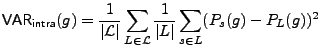
Intuitively, this measures the average distance between the probability of g for
given a speaker and the probability of g given that speaker's language; i.e., the
average variance of the probability distributions PL(g). We compute
the interclass variability as:
 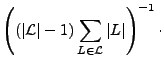 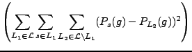
This measures, on average, the difference between the probability of g for a given
speaker and the probability of g given every other language. The second two summations
in the second term measure the distance from each speaker in a specific language to the
means of all other languages. The first summation and the leading normalization term
are used to compute the average over all languages. As an example, if we consider the
seventh and eighth bins in the unigram case illustrated in Figure
2, then VARinter(15
.0 kbps)
< VARinter(18.
2 kbps).
We set the overall distinguishability for n-gram g to be DIS(g) = VARinter(g) / VARintra(g). Intuitively, if DIS(g) is large, then speakers of the same language tend to have similar probability densities for g, and these densities will vary across languages. We choose to make our classification decisions using only those g with DIS(g) > 1, we denote this set of distinguishing n-grams as G. The model for language L is simply the probability distribution PL over G.
To further refine the models, we remove outliers (speakers) who might contribute noise to each distribution. In order to do this, we must first specify a distance metric between a speaker s and a language L. Suppose that we extract N total n-grams from s's speech samples. Then, we compute the distance between s and L as:
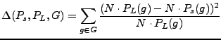
We then remove the speakers s from L for which D(Ps,PL,G) is greater than some language-specific threshold tL. After we have removed these outliers, we recompute PL with the remaining speakers.
Given our refined models, our goal is to use a speaker's samples to identify the speaker's language. We assign the speaker s to the language with the model that is closest to the speaker's distribution over G as follows:
To determine the accuracy of our classifier, we apply the standard
leave-one-out cross validation analysis to each speaker in our data
set. That is, for a given speaker, we remove that speaker's samples and use the remaining
samples to compute G and the models PL for each language in L � L. We choose the tL such that 15% of the speakers are removed as outliers (these outliers are eliminated during model creation, but they are still included in classification results). Next, we compute the probability distribution, Ps, over G using
the speaker's samples. Finally, we classify the speaker using Ps
and the outlier-reduced models derived from the other speakers in the corpus.
4 Empirical Evaluation
To evaluate the performance of our classifier in a realistic
environment, we simulated VoIP calls for many different languages by
playing audio files from the Oregon Graduate Institute Center for
Speech Learning & Understanding's "22 Language" telephone speech
corpus [15] over a VoIP connection.
This corpus is widely used in language identification studies in the speech
recognition community (e.g. [19], [33]).
It contains recordings from a total of 2066 native speakers of 21 languages,
with over 3 minutes of audio per speaker. The data was originally collected
by having users call in to an automated telephone system that prompted
them to speak about several topics and recorded their responses. There
are several files for each user. In some, the user was asked to answer
a question such as "Describe your most recent meal" or "What is
your address?" In others, they were prompted to speak freely for up
to one minute. This type of free-form speech is especially appealing for
our evaluation because it more accurately represents the type of speech
that would occur in a real telephone conversation. In other files, the
user was prompted to speak in English or was asked about the language(s)
they speak. To avoid any bias in our results, we omit these files from
our analysis, leaving over 2 minutes of audio for each user.
See Appendix A for specifics concerning the dataset.
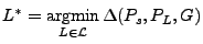
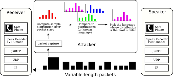 Figure 6: Experimental setup.
Our experimental setup includes two PC's running Linux with open
source VoIP software [17]. One of the machines acts as a
server and listens on the network for SIP calls. Upon receiving a call,
it automatically answers and negotiates the setup of the voice channel
using Speex over RTP. When the voice channel is established, the
server plays a file from the corpus over the connection to the caller,
and then terminates the connection. The caller, which is another
machine on our LAN, automatically dials the SIP address of the server
and then "listens" to the file the server plays, while recording the
sequence of packets sent from the server. The experimental setup is
depicted in Figure 6.
Although our current evaluation is based on data collected on a local
area network, we believe that languages could be identified under most or
all network conditions where VoIP is practical. First, RTP (and SRTP)
sends in the clear a timestamp corresponding to the sampling time of
the first byte in the packet data [25]. This timestamp can
therefore be used to infer packet ordering and identify packet loss.
Second, VoIP is known to degrade significantly under undesirable network
connections with latency more than a few hundred milliseconds
[11], and it is also sensitive to packet loss
[13]. Therefore any network which allows for
acceptable call quality should also give our classifier a sufficient
number of trigrams to make an accurate classification.
For a concrete test of our techniques on wide-area network data, we
performed a smaller version of the above experiment by playing a reduced
set of 6 languages across the Internet between a server on our LAN and a
client machine on a residential DSL connection. In the WAN traces, we
observed less than 1% packet loss, and there was no statistically
significant difference in recognition rates for the LAN and WAN
experiments.
4.1 Classifier Accuracy
In what follows, we examine the classifier's performance when
trained using all available samples (excluding, of course, the target
user's samples). To do so, we test each speaker against all 21
models.
The results are presented in
Figures 7 and 8.
Figure 7 shows the confusion matrix resulting from
the tests. The x axis specifies the language of the speaker, and
the y axis specifies the language of the model. The density of the
square at position (x,y) indicates how often samples from speakers
of language x were classified as belonging to language y.
 Figure 7: Confusion Matrix for 21-way test using trigrams. Darkest and lightest boxes represent accuracies of 0.4 and 0.0, respectively.
|
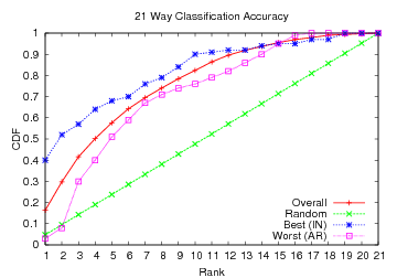 Figure 8: CDF showing how often the speaker's language was among
the classifier's top x choices.
Figure 8: CDF showing how often the speaker's language was among
the classifier's top x choices.
|
To grasp the significance of our results, it is important to note that
if packet lengths leaked no information, then the classification rates
for each language would be close to random, or about 4.8%. However,
the confusion matrix shows a general density along the y = x
line. The classifier performed best on Indonesian (IN) which is
accurately classified 40% of the time (an eight fold improvement over random guessing). It also performed well on
Russian (RU), Tamil (TA), Hindi (HI), and Korean (KO), classifying at
rates of 35, 35, 29 and 25 percent, respectively. Of course,
Figure 7 also shows that in several instances,
misclassification occurs. For instance, as noted in
Figure 2, English (EN) and Brazilian Portuguese (BP) exhibit similar unigram distributions, and indeed when
misclassified, English was often confused with
Brazilian Portuguese (14% of the time). Nonetheless, we believe these results
are noteworthy, as if VoIP did not leak information, the
classification rates would be close to those of random guessing. Clearly, this is not the case, and our overall accuracy was
16.3%-that is, a three and a half fold improvement over random guessing.
An alternative perspective is given in Figure 8, which
shows how often the speaker's language was among the
classifier's top x choices. We plot random guessing as a baseline,
along with languages that exhibited the highest and lowest
classification rates. On average, the correct language was among our
top four speculations 50.2% of the time. Note the significant improvement over random guessing, which would only place the correct language in the top four choices approximately 19% of the time. Indonesian is correctly
classified in our top three choices 57% of the time, and even
Arabic-the language with the lowest overall classification
rates-was correctly placed among our top three choices 30% of the
time.
In many cases, it might be worthwhile to distinguish between only two
languages, e.g., whether an encrypted conversation in English or Spanish.
We performed tests that aimed at identifying the correct language when
supplied only two possible choices.
We see a stark improvement over random guessing, with seventy-five percent
of the language combinations correctly distinguished with an accuracy
greater than 70.1%; twenty-five percent had accuracies greater than 80%.
Our overall binary classification rate was 75.1%.
Our preliminary findings in Section 2 are strongly correlated
to our empirical results. For example, rates for Russian versus Italian
and Mandarin versus Tamil (see Figure 5) were
78.5% and 84%, respectively. The differences in the histograms shown
earlier (Figure 2) also have direct implications for
our classification rates in this case. For instance, our classifier's
accuracy when tasked with distinguishing between Brazilian Portuguese
and English was only 66.5%, whereas the accuracy for English versus
Hungarian was 86%.
4.2 Reducing Dimensionality to Improve Performance
Although these results adequately demonstrate that length-preserving
encryption leaks information in VoIP, there are limiting factors to
the aforementioned approach that hinder classification accuracy. The primary
difficulty arises from the fact that the classifier represents each
speaker and language as a probability distribution over a very high
dimensional space. Given 9 different observed packet lengths, there
are 729 possible different trigrams. Of these possibilities, there
are 451 trigrams that are useful for classification, i.e.,
DIS(g) > 1
(see Section 3). Thus, speaker and language
models are probability distributions over a 451-dimensional space.
Unfortunately, given our current data set of approximately 7,277
trigrams per speaker, it is difficult to estimate densities over
such a large space with high precision.
One way to address this problem is based on the observation that some
bit rates are used in similar ways by the Speex encoder. For example,
the two lowest bit rates, which result in packets of 41 and 46 bytes,
respectively, are often used to encode periods of silence or non-speech.
Therefore, we can reasonably consider the two smallest packet sizes
functionally equivalent and put them together into a single group.
In the same way, other packet sizes may be used similarly enough to warrant
grouping them together as well. We experimented with several mappings
of packet sizes to groups, but found that the strongest results are
obtained by mapping the two smallest packet lengths together, mapping
all of the mid-range packet lengths together, and leaving the largest
packet size in a group by itself.
We assign each group a specific symbol, s, and then compute n-grams
from these symbols instead of the original packet sizes. So, for
example, given the sequence of packet lengths 41, 50, 46, and 55,
we map 41 and 46 to s1 and 50 and 55 to s2 to extract the
3-grams (s1, s2, s1) and (s2, s1, s2), etc.
Our classification process then continues as before, except that the
reduction in the number of symbols allows us to expand our
analysis to 4-grams. After removing the 4-grams g with
DIS(g) < 1, we are left with 47 different 4-gram combinations.
Thus, we reduced the dimensionality of the points from 451 to 47. Here
we are estimating distributions over a 47-dimensional space using on
average of 7,258 4-grams per speaker.
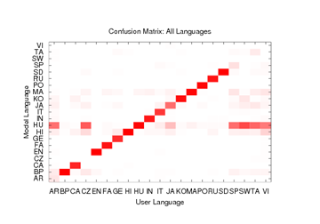 Figure 9: Confusion Matrix for the 21-way test using 4-grams and reduced set of symbols. Darkest and lightest boxes represent accuracies of 1.0 and 0.0, respectively.
|
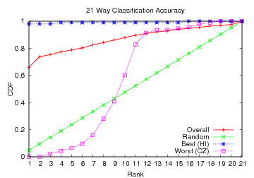 Figure 10: CDF showing how often the speaker's language was among
the classifier's top x choices using 4-grams and reduced set of symbols.
Figure 10: CDF showing how often the speaker's language was among
the classifier's top x choices using 4-grams and reduced set of symbols.
|
Results for this classifier are shown in Figures 9
and 10. With these improvements, the 21-way
classifier correctly identifies the language spoken 66% of the time-a
fourfold improvement over our original classifier and more than 13 times
better than random guessing. It recognizes 14 of the 21
languages exceptionally well, identifying them with over 90% accuracy.
At the same time, there is a small group of languages which the
new classifier is not able to identify reliably; Czech, Spanish,
and Vietnamese are never identified correctly on the first try.
This occurs mainly because the languages which are not recognized
accurately are often misidentified as one of a handful of other
languages. Hungarian, in particular, has false positives on
speakers of Arabic, Czech, Spanish, Swahili, Tamil, and Vietnamese.
These same languages are also less frequently misidentified as
Brazilian Portuguese, Hindi, Japanese, Korean, or Mandarin.
In future work, we plan to investigate what specific acoustic features
of language cause this classifier to perform so well on many of the
languages while failing to accurately recognize others.
Binary classification rates, shown in Figure 11
and Table 1, are similarly improved over our initial
results. Overall, the classifier achieves over 86% accuracy when
distinguishing between two languages. The median accuracy is 92.7%
and 12% of the language pairs can be distinguished at rates greater
than 98%. In a few cases like Portuguese versus Korean or Farsi versus
Polish, the classifier exhibited 100% accuracy on our test data.
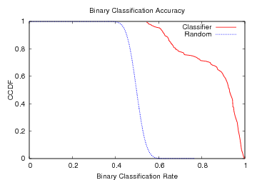 Figure 11: CCDF for overall accuracy of the binary classifier using 4-grams and reduced set of symbols.
|
| Lang. | Acc. | | Lang. | Acc | |
| EN-FA | 0.980 | | CZ-JA | 0.544 |
| GE-RU | 0.985 | | AR-SW | 0.549 |
| FA-SD | 0.990 | | CZ-HU | 0.554 |
| IN-PO | 0.990 | | CZ-SD | 0.554 |
| PO-RU | 0.990 | | MA-VI | 0.565 |
| BP-PO | 0.995 | | JA-SW | 0.566 |
| EN-HI | 0.995 | | HU-VI | 0.575 |
| HI-PO | 0.995 | | CZ-MA | 0.580 |
| BP-KO | 1.000 | | CZ-SW | 0.590 |
| FA-PO | 1.000 | | HU-TA | 0.605 |
Table 1: Binary classifier recognition rates for selected language pairs.
Languages and their abbreviations are listed in Appendix A.
|
Interestingly, the results of our classifiers are comparable to
those presented by Zissman [38] in an early
study of language identification techniques using full acoustic data.
Zissman implemented and compared four different language recognition techniques, including
Gaussian mixture model (GMM) classification and techniques based on
single-language phone recognition and n-gram language modeling.
All four techniques used cepstral coefficients as input [22].
The GMM classifier described by Zissman is much simpler than the other techniques and
serves primarily as a baseline for comparing the performance of the
more sophisticated methods presented in that work. Its accuracy is
quite close to that of our initial classifier: with access to
approximately 10 seconds of raw acoustic data, it scored approximately
78% for three language pairs, compared to our classifer's 89%.
The more sophisticated classifiers in [38] have
performance closer to that of our improved classifier. In particular,
an 11-way classifier based on phoneme recognition and n-gram language
modeling (PRLM) was shown to achieve 89% accuracy when given 45s of
acoustic data. In each case, our classifier has the advantage of a
larger sample, using around 2 minutes of data.
Naturally, current techniques for language identification have improved
on the earlier work of Zissman and others, and modern error rates are
almost an order of magnitude better than what our classifiers achieve.
Nevertheless, this comparison serves to demonstrate the point that we
are able to extract significant information from encrypted VoIP packets,
and are able to do so with an accuracy close to a reasonable classifier
with access to acoustic data.
Discussion
We note that since the audio files in our corpus were recorded over a
standard telephone line, they are sampled at 8kHz and encoded as
16-bit PCM audio, which is appropriate for Speex narrowband mode. While almost all
traditional telephony samples the source audio at 8kHz, many soft
phones and VoIP codecs have the ability to use higher sampling rates
such as 16kHz or 32kHz to achieve better audio quality at the tradeoff
of greater load on the network. Unfortunately, without a higher-fidelity
data set, we have been unable to evaluate our techniques on VoIP
calls made with these higher sampling rates.
Nevertheless, we feel that the results we derive from
using the current training set are also informative for higher-bandwidth
codecs for two reasons.
First, it is not uncommon for regular phone conversations to be
converted to VoIP, enforcing the use of an 8kHz sampling rate.
Our test setup accurately models the
traffic produced under this scenario. Second, and more importantly,
by operating at the 8kHz level, we argue that we work with less
information about the underlying speech, as we are only able to
estimate bit rates up to a limited fidelity. Speex wideband mode, for
example, operates on speech sampled at 16kHz and in VBR mode uses a
wider range of bit rates than does the narrowband mode. With access
to more distinct bit rates, one would expect to be able to extract
more intricate characteristics about the underlying speech. In that
regard, we believe that our results could be further improved given
access to higher-fidelity samples.
4.3 Mitigation
Recall that these results are possible because the default mode of encryption
in SRTP is to use a length-preserving stream cipher. However, the official
standard [4] does allow implementations to optionally pad the plaintext payload
to the next multiple of the cipher's block size, so that the original
payload size is obscured. Therefore, we investigate the effectiveness of
padding against our attack, using several block sizes.
To determine the packet sizes that would be produced by encryption with
padding, we simply modify the packet sizes we observed in our network
traces by increasing their RTP payload sizes to the next multiple of the
cipher's block size. To see how our attack is affected by this padding,
we re-ran our experiments using block sizes of 128, 192, 256, and 512 bits.
Padding to a block size of 128 bits results in 4 distinct packet sizes; this number
decreases to 3 distinct sizes with 192-bit blocks, 2 sizes with 256-bit
blocks, and finally, with 512-bit blocks, all packets are the same size.
Figure 12 shows the CDF for the classifier's results for
these four cases, compared to random guessing and to the results we achieve
when there is no padding.
Padding to 128-bit blocks is largely ineffective because there is still
sufficient granularity in the packet sizes that we can map them to basically
to the same three bins used by our improved classifier in Section 4.2.
Even with 192- or 256-bit blocks, where dimensionality reduction does not
offer substantial improvement, the correct language can be identified on the first
guess over 27% of the time-more than 5 times better than random guessing.
It is apparent from these results that, for encryption with padding to be
an effective defense against this type of information leakage, the block
size must be large enough that all encrypted packets are the same size.
Relying on the cryptographic layer to protect against both eavesdropping
and traffic analysis has a certain philosophical appeal because then the
compression layer does not have to be concerned with security issues.
On the other hand, padding incurs significant overhead in the number of
bytes that must be transmitted. Table 2 lists the
increase in traffic volume that arises from padding to each block size,
as well as the improvement of the overall accuracy of the classifier over
random guessing.
| | | | Improvement |
| | | vs Random | |
| none | 0.0% | 66.0% | 13.8x |
| 128 bits | 8.7% | 62.5% | 13.0x |
| 192 bits | 13.8% | 27.1% | 5.7x |
| 256 bits | 23.9% | 27.2% | 5.7x |
| 512 bits | 42.2% | 6.9% | 1.4x |
Table 2: Tradeoff of effectiveness versus overhead incurred for padding VoIP packets to various block sizes.
|
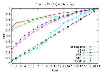 Figure 12: The effect of padding on classifier accuracy.
|
Another solution for ensuring that there is no information leakage is
to use a constant bit rate codec, such as Speex in CBR mode, to send
packets of fixed length. Forcing the encoder to use a fixed number of
bits is an attractive approach, as the encoder could use the bits that
would otherwise be used as padding to improve the quality of the encoded
sound. While both of these approaches would detract from the bandwidth
savings provided by VBR encoders, they provide much stronger privacy
guarantees for the participants of a VoIP call.
5 Related Work
Some closely related work is that of Wang et al.
[31] on tracking VoIP calls over low-latency
anonymizing networks such as Tor [9]. Unlike our analysis,
which is entirely passive, the attack in [31]
requires that the attacker be able to actively inject delays
into the stream of packets as they traverse the anonymized network.
Other recent work has explored extracting sensitive information from
several different kinds of encrypted network connections. Sun et al.
[27], for example, examined World Wide Web traffic
transmitted in HTTP over secure (SSL) connections and were able to
identify a set of sensitive websites based on the number and sizes of
objects in each encrypted HTTP response. Song et al.
[26] used packet interarrival times to infer
keystroke patterns and ultimately crack passwords typed over SSH.
Zhang and Paxson [36] also used packet timing
in SSH traffic to identify pairs of connections which form part of a
chain of "stepping stone" hosts between the attacker and his
eventual victim. In addition to these application-specific attacks,
our own previous work demonstrates that packet size and timing are
indicative of the application protocol used in SSL-encrypted TCP
connections and in simple forms of encrypted tunnels
[34].
Techniques for autmatically identifying spoken languages were the
subject of a great deal of work in the mid
1990's [18,38]. While these
works used a wide range of features extracted from the audio data and
employed many different machine learning techniques, they all
represent attempts to mimic the way humans differentiate between
languages, based on differences in the sounds produced. Because our
classifier does not have direct access to the acoustic data, it is
unrealistic to expect that it could outperform a modern language
recognition system, where error rates in the single digits are not
uncommon.
Nevertheless, automatic language identification is not considered a
solved problem, even with access to full acoustic data, and work is
ongoing in the speech community to improve recognition rates and
explore new approaches (see, e.g.,
[32,8,1]).
6 Conclusions
In this paper, we show that despite efforts devoted to securing
conversations that traverse Voice over IP, an adversary can still
exploit packet lengths to discern considerable information about the
underlying spoken language. Our techniques examine patterns in the
output of Variable Bit Rate encoders to infer characteristics of the
encoded speech. Using these characteristics, we evaluate our
techniques on a large corpus of traffic from different speakers, and
show that our techniques can classify (with reasonable accuracy) the
language of the target speaker. Of the 21 languages we evaluated, we
are able to correctly identify 14 with accuracy greater than
90%. When tasked with distinguishing between just two languages,
our average accuracy over all language pairs is greater than 86%.
These recognition rates are on par with early results from the language
identification community, and they demonstrate that variable bit rate coding
leaks significant information. Moreover, we show that simple padding
is insufficient to prevent leakage of information about the language
spoken. We believe that this information leakage from encrypted VoIP
packets is a significant privacy concern. Fortunately, we are able
to suggest simple remedies that would thwart our attacks.
Acknowledgments
We thank Scott Coull for helpful conversations throughout the course
of this research, as well as for pointing out the linphone application
[17]. We also thank Patrick McDaniel and Patrick Traynor
for their insightful comments on early versions of this work. This
work was funded in part by NSF grants CNS-0546350 and CNS-0430338.
References
- [1]
-
NIST language recognition evaluation.
http://www.nist.gov/speech/tests/lang/index.htm.
- [2]
-
S. Andersen, A. Duric, H. Astrom, R. Hagen, W. Kleijn, and J. Linden.
Internet Low Bit Rate Codec (iLBC), 2004.
RFC 3951.
- [3]
-
R. Barbieri, D. Bruschi, and E. Rosti.
Voice over IPsec: Analysis and solutions.
In Proceedings of the 18th Annual Computer Security Applications
Conference, pages 261-270, December 2002.
- [4]
-
M. Baugher, D. McGrew, M. Naslund, E. Carrara, and K. Norrman.
The secure real-time transport protocol (SRTP).
RFC 3711.
- [5]
-
F. Beritelli.
High quality multi-rate CELP speech coding for wireless ATM
networks.
In Proceedings of the 1998 Global Telecommunications
Conference, volume 3, pages 1350-1355, November 1998.
- [6]
-
P. Biondi and F. Desclaux.
Silver needle in the Skype.
In BlackHat Europe, 2006.
http://www.blackhat.com/presentations/bh-europe-06/bh-eu-06-biondi/bh-eu-06-biondi-up.pdf.
- [7]
-
M. Blaze.
Protocol failure in the escrowed encryption standard.
In Proceedings of Second ACM Conference on Computer and
Communications Security, pages 59-67, 1994.
- [8]
-
L. Burget, P. Matejka, and J. Cernocky.
Discriminative training techniques for acoustic language
identification.
In Proceedings of the 2006 IEEE International Conference on
Acoustics, Speech, and Signal Processing, volume 1, pages
I-209-I-212, May 2006.
- [9]
-
R. Dingledine, N. Mathewson, and P. Syverson.
Tor: The second-generation onion router.
In Proceedings of the 13th USENIX Security Symposium,
pages 303-320, August 2004.
- [10]
-
International Telecommunications Union.
Recommendation G.711: Pulse code modulation (PCM) of voice
frequencies, 1988.
- [11]
-
International Telecommunications Union.
Recommendation P.1010: Fundamental voice transmission objectives
for VoIP terminals and gateways, 2004.
- [12]
-
International Telecommunications Union.
Recommendation G.729: Coding of speech at 8 kbits using
conjugate-structure algebraic-code-excited linear prediction (CS-ACELP),
2007.
- [13]
-
W. Jiang and H. Schulzrinne.
Modeling of packet loss and delay and their effect on real-time
multimedia service quality.
In Proceedings of the 10th International Workshop on
Network and Operating System Support for Digital Audio and Video, June 2000.
- [14]
-
D. R. Kuhn, T. J. Walsh, and S. Fries.
Security considerations for voice over IP systems.
Technical Report Special Publication 008-58, NIST, January 2005.
- [15]
-
T. Lander, R. A. Cole, B. T. Oshika, and M. Noel.
The OGI 22 language telephone speech corpus.
In EUROSPEECH, pages 817-820, 1995.
- [16]
-
S. McClellan and J. D. Gibson.
Variable-rate CELP based on subband flatness.
IEEE Transactions on Speech and Audio Processing,
5(2):120-130, March 1997.
- [17]
-
S. Morlat.
Linphone, an open-source SIP video phone for Linux and Windows.
http://www.linphone.org/.
- [18]
-
Y. K. Muthusamy, E. Barnard, and R. A. Cole.
Reviewing automatic language identification.
IEEE Signal Processing Magazine, 11(4):33-41, October 1994.
- [19]
-
J. Navrátil.
Spoken language recognition-a step toward multilinguality in
speechprocessing.
IEEE Transactions on Speech and Audio Processing,
9(6):678-685, September 2001.
- [20]
-
E. Paksoy, A. McCree, and V. Viswanathan.
A variable rate multimodal speech coder with gain-matched
analysis-by-synthesis.
In Proceedings of the 1997 IEEE International Conference on
Acoustics, Speech, and Signal Processing, volume 2, pages 751-754, April
1997.
- [21]
-
N. Provos.
Voice over misconfigured internet telephones.
http://vomit.xtdnet.nl.
- [22]
-
L. Rabiner and B. Juang.
Fundamentals of Speech Recognition.
Prentice Hall, 1993.
- [23]
-
J. Rosenberg, H. Schulzrinne, G. Camarillo, A. Johnston, J. Peterson,
R. Sparks, M. Handley, and E. Schooler.
SIP: Session initiation protocol.
RFC 3261.
- [24]
-
M. R. Schroeder and B. S. Atal.
Code-excited linear prediction(CELP): High-quality speech at very
low bit rates.
In Proceedings of the 1985 IEEE International Conference on
Acoustics, Speech, and Signal Processing, volume 10, pages 937-940, April
1985.
- [25]
-
H. Schulzrinne, S. Casner, R. Frederick, and V. Jacobson.
RTP: A transport protocol for real-time applications.
RFC 1889.
- [26]
-
D. Song, D. Wagner, and X. Tian.
Timing analysis of keystrokes and SSH timing attacks.
In Proceedings of the 10th USENIX Security Symposium,
August 2001.
- [27]
-
Q. Sun, D. R. Simon, Y.-M. Wang, W. Russell, V. N. Padmanabhan, and L. Qiu.
Statistical identification of encrypted web browsing traffic.
In Proceedings of the IEEE Symposium on Security and Privacy,
pages 19-30, May 2002.
- [28]
-
J.-M. Valin.
The Speex codec manual.
http://www.speex.org/docs/manual/speex-manual.pdf, August 2006.
- [29]
-
J.-M. Valin and C. Montgomery.
Improved noise weighting in CELP coding of speech - applying the
Vorbis psychoacoustic model to Speex.
In Audio Engineering Society Convention, May 2006.
See also http://www.speex.org.
- [30]
-
S. V. Vaseghi.
Finite state CELP for variable rate speech coding.
IEE Proceedings I Communications, Speech and Vision,
138(6):603-610, December 1991.
- [31]
-
X. Wang, S. Chen, and S. Jajodia.
Tracking anonymous peer-to-peer VoIP calls on the Internet.
In Proceedings of the 12th ACM conference on Computer and
communications security, pages 81-91, November 2005.
- [32]
-
C. White, I. Shafran, and J.-L. Gauvain.
Discriminative classifiers for language recognition.
In Proceedings of the 2006 IEEE International Conference on
Acoustics, Speech, and Signal Processing, volume 1, pages
I-213-I-216, May 2006.
- [33]
-
E. Wong, T. Martin, T. Svendsen, and S. Sridharan.
Multilingual phone clustering for recognition of spontaneous
indonesian speech utilising pronunciation modelling techniques.
In Proceedings of the 8th European Conference on Speech
Communication and Technology, pages 3133-3136, September 2003.
- [34]
-
C. V. Wright, F. Monrose, and G. M. Masson.
On inferring application protocol behaviors in encrypted network
traffic.
Journal of Machine Learning Research, 7:2745-2769, December
2006.
Special Topic on Machine Learning for Computer Security.
- [35]
-
L. Zhang, T. Wang, and V. Cuperman.
A CELP variable rate speech codec with low average rate.
In Proceedings of the 1997 IEEE International Conference on
Acoustics, Speech, and Signal Processing, volume 2, pages 735-738, April
1997.
- [36]
-
Y. Zhang and V. Paxson.
Detecting stepping stones.
In Proceedings of the 9th USENIX Security Symposium, pages
171-184, August 2000.
- [37]
-
P. Zimmermann, A. Johnston, and J. Callas.
ZRTP: Extensions to RTP for Diffie-Hellman key agreement for
SRTP, March 2006.
IETF Internet Draft.
- [38]
-
M. A. Zissman.
Comparison of four approaches to automatic language identification of
telephone speech.
IEEE Transactions on Speech and Audio Processing, 4(1),
January 1996.
A Data Set Breakdown
The empirical analysis performed in this paper is based on one of the
most widely used data sets in the language recognition community. The
Oregon Graduate Institute CSLU 22 Language corpus provides speech
samples from 2,066 native speakers of 21 distinct languages. Indeed,
the work of Zissman [38] that we analyze in
Section 4 used an earlier version of this corpus.
Table 3 provides some statistics about the data set.
| | | | Minutes |
| | | per Speaker | |
| Arabic | AR | 100 | 2.16 |
| Br. Portuguese | BP | 100 | 2.52 |
| Cantonese | CA | 93 | 2.63 |
| Czech | CZ | 100 | 2.02 |
| English | EN | 100 | 2.51 |
| Farsi | FA | 100 | 2.57 |
| German | GE | 100 | 2.33 |
| Hindi | HI | 100 | 2.74 |
| Hungarian | HU | 100 | 2.81 |
| Indonesian | IN | 100 | 2.45 |
| Italian | IT | 100 | 2.25 |
| Japanese | JA | 100 | 2.33 |
| Korean | KO | 100 | 2.58 |
| Mandarin | MA | 100 | 2.75 |
| Polish | PO | 100 | 2.64 |
| Russian | RU | 100 | 2.55 |
| Spanish | SP | 100 | 2.76 |
| Swahili | SW | 73 | 2.26 |
| Swedish | SD | 100 | 2.23 |
| Tamil | TA | 100 | 2.12 |
| Vietnamese | VI | 100 | 1.96 |
Table 3: Statistics about each language in our data set [15]. Minutes of speech is measured how many of minutes of speech we used during our tests.
|