2007 USENIX Annual Technical Conference
Pp. 171–184 of the Proceedings
Using Provenance to Aid in Personal File Search
Sam Shah⋆ Craig A. N. Soules † Gregory R. Ganger‡ Brian D. Noble⋆
⋆
University of Michigan †HP Labs ‡Carnegie Mellon University
As the scope of personal data grows, it becomes increasingly
difficult to find what we need when we need it. Desktop
search tools provide a potential answer, but most existing
tools are incomplete solutions: they index content, but
fail to capture dynamic relationships from the user’s
context. One emerging solution to this is context-enhanced
search, a technique that reorders and extends the results of
content-only search using contextual information. Within this
framework, we propose using strict causality, rather than
temporal locality, the current state of the art, to direct
contextual searches. Causality more accurately identifies data
flow between files, reducing the false-positives created by
context-switching and background noise. Further, unlike
previous work, we conduct an online user study with a
fully-functioning implementation to evaluate user-perceived
search quality directly. Search results generated by our
causality mechanism are rated a statistically-significant
17% higher on average over all queries than by using
content-only search or context-enhanced search with
temporal locality.
1 Introduction
Personal data has become increasingly hard to manage, find,
and retrieve as its scope has grown. As storage capacity
continues to increase, the number of files belonging to an
individual user, whether a home or corporate desktop user,
has increased accordingly [7]. The principle challenge is no
longer efficiently storing this data, but rather organizing it.
To reduce the friction users experience in finding their data,
many personal search tools have emerged. These tools build
a content index and allow keyword search across this
index. Despite their growing prevalence, most of these tools are,
however, incomplete solutions: they index content, not
context. They capture only static, syntactic relationships, not
dynamic, semantic ones. To see why this is important,
consider the difference between compiler optimization
and branch prediction. The compiler has access only to
the code, while the processor can see how that code is
commonly used. Just as run-time information leads to
significant performance optimizations, users find contextual
and semantic information useful in searching their own
repositories [22].
Context-enhanced search is beginning to receive attention,
but it is unclear what dynamic information is most useful in
assisting search. Soules and Ganger [21] developed a
system, named Connections, that uses temporal locality to
capture the provenance of data: for each new file written, the
set of files read “recently” form a kinship or relation
graph, which Connections uses to extend search results
generated by traditional static, content-based indexing
tools. Temporal locality is likely to capture many true
relationships, but may also capture spurious, coincidental
ones. For example, a user who listens to music while
authoring a document in her word processor may or may not
consider the two “related” when searching for a specific
document.
To capture the benefit of temporal locality while avoiding
its pitfall, we provide a different mechanism to deduce
provenance: causality. That is, we use data flow through and
between applications to impart a more accurate relation
graph. We show that this yields more desirable search results
than either content-only indexing or kinship induced by
temporal locality.
Our context-enhancing search has been implemented
for Windows platforms. As part of our evaluation, we
conduct a user study with this prototype implementation
to measure a user’s perceived search quality directly.
To accomplish this, we adapt two common techniques
from the social sciences and human-computer interaction
to the area of personal file search. First, we conduct
a randomized, controlled trial to gauge the end-to-end
effects of our indexing technique. Second, we conduct
a repeated measures experiment, where users evaluate the
different indexing techniques side-by-side, locally on their
own machines. This style of experiment is methodogically
superior as it measures quality directly while preserving
privacy of user data and actions.
The results indicate that our causal provenance algorithm
fares better than using temporal locality or pure content-only
search, being rated a statistically-significant 17% higher, on
average, than the other algorithms by users with minimal
space and time overheads. Further, as part of our study,
we also provide some statistics about personal search
behavior.
The contributions of this paper are:
- The identification of causality as a useful
mechanism to inform contextual indexing tools and
a description of a prototype system for capturing it.
- An exploration of the search behavior of a
population of 27 users over a period of one month.
- A user study, including a methodology for
evaluating personal search systems, demonstrating
that causality-enhanced indexing provides higher
quality search results than either those based on
temporal locality or those using content information
only.
The remainder of this paper is organized as follows. In
Section 2, we give an overview of related work. Section 3
describes how our system deduces and uses kinship
relationships, with Section 4 outlining our prototype
implementation. Section 5 motivates and presents our
evaluation and user study and Section 6 explores the search
behavior of our sample population. Finally, Section 7
concludes.
2 Related Work
There are various static indexing tools for one’s filespace.
Instead of strict hierarchal naming, the semantic file
system [10] allows assignment of attributes to files,
facilitating search over these attributes. Since most users are
averse to ascribing keywords to their files, the semantic
file system provides transducers to distill file contents
into keywords. The semantic file system focuses on the
mechanism to store attributes, not on content analysis to
distill these attributes.
There are several content-based search tools available
today, including Google Desktop Search, Windows Desktop
Search and Yahoo! Desktop Search, among others.
These systems extract a file’s content into an index, permitting search across this index. While the details of
such systems are opaque, it is likely they use forefront
technologies from the information retrieval community.
Several such advanced research systems exist, Indri [1]
being a prime example. These tools are orthogonal to our
system in that they all analyze static data with well-defined
types to generate an index, ignoring crucial contextual
information that establishes semantic relationships between
files.
The seminal work in using gathered context to aid in file
search is by Soules and Ganger [21] in the form of a file
system search tool named Connections. Connections
identifies temporal relationships between files and uses that
information to expand and reorder traditional content-only
search results, improving average precision and recall
compared to Indri. We use some component algorithms from
Connections (§3.2) and compare against its temporal locality
approach (§3.1.1).
Our notion of provenance is a subset of that used by the
provenance-aware storage system (PASS) [17]. PASS
attempts to capture a complete lineage of a file, including the
system environment and user- and application-specified
annotations of provenance. A PASS filesystem, if available,
would negate the need for our relation graph. Indeed, the
technique used by PASS to capture system-level provenance
is very similar to our causality algorithm (§3.1.2).
Several systems leverage other forms of context for file
organization and search. Phlat [5] is a user interface for
personal search, running on Windows Desktop Search, that
also provides a mechanism for tagging or classifying
of data. The user can search and filter by contextual
cues such as date and person. Our system provides a
simpler UI, permitting search by keywords only (§4), but
could use Phlat’s interface in the future. Another system,
called “Stuff I’ve Seen” [8], remembers previously seen
information, providing an interface that allows a user to
search their historical information using contextual cues.
The Haystack project [12] is a personal information
manager that organizes data, and operations on data, in a
context-sensitive manner. Lifestreams [9] provides an
interface that uses time as its indexing and presentation
mechanism, essentially ordering results by last access time.
Our provenance techniques could enhance these systems
through automated clustering of semantically-related
items.
3 Architecture
Our architecture matches that of Soules and Ganger [21]: we
augment traditional content search using kinship relations
between files. After the user enters keywords in our search
tool, the tool runs traditional content-only search using those
keywords—the content-only phase—and then uses the
previously constructed relation graph to reorder these results
and identify additional hits—the context-enhancing
phase. These new results are then returned to the user.
Background tasks run on the user’s machine to periodically
index a file’s content for the content-only phase and to
monitor system events to build the relation graph for the
context-enhancing phase. This section describes how the
system deduces and uses these relationships to re-rank
results.
3.1 Inferring Kinship Relationships
A kinship relation, f → f ′ where f and f ′ are files on a
user’s system, indicates that f is an ancestor of f ′, implying
that f may have played a role in the origin of f ′. These
relationships are encoded in the relation graph, which is used
to reorder and extend search results in the context-enhancing
phase.
We evaluate two methods of deducing these kinship
relations: temporal locality and causality. Both methods
classify the source file of a read as input and the destination
file of a write as output by inferring user task behavior from
observed actions.
3.1.1 Temporal Locality Algorithm
The temporal locality algorithm, as employed in
Soules and Ganger [21], infers relations by maintaining a
sliding relation window of files accessed within the previous
t seconds system-wide. Any write operation within this
window is tied to any previous read operation within the
window. This is known as the read/write operational filter
with directed links in Soules and Ganger [21], which was
found the most effective of several considered.
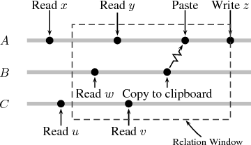
Consider the sequence of system events shown in
Figure 1. There are three processes, A, B, and C, running
concurrently. C reads files u and v, A reads files x and y. B
reads w and copies data to A through a clipboard IPC action
initiated by the user. Following this, A then writes file
z.
The relation window at z’s write contains reads of y, w,
and v. The temporal locality algorithm is process agnostic
and views reads and writes system-wide, distinguishing only
between users. The algorithm thus returns the relations
{y → z,w → z,v → z}.
The relation window attempts to capture the transient
nature of a user task. Too long a window will cause unrelated
tasks to be grouped, but too short a window will cause
relationships to be missed.
3.1.2 Causality Algorithm
Rather than using a sliding window to deduce user tasks, this
paper proposes viewing each process as a filter that mutates
its input to produce some output. This causality algorithm
tracks how input flows—at the granularity of processes—to
construct kinship relations, determining what output is
causally related to which inputs.
Specifically, whenever a write event occurs, the following
relations are formed:
(a) Any previous files read within the same process are
tied to the current file being written;
(b) Further, the algorithm tracks IPC transmits and
its corresponding receives, forming additional
relationships by assessing the transitive closure
of file system events formed across these IPC
boundaries. That is, for each relation f → f ′, there is a directed left-to-right
path in the time diagram starting at a read event of file f and
ending at the write of file f ′. There is no temporal bound
within this algorithm.
Reconsidering Figure 1, A reads x and y to generate z; the
causality algorithm produces the relations {x → z,y → z}
via condition (a). B produces no output files given its read
of w, but the copy-and-paste operation represents an IPC
transmit from B with a corresponding receive in A. By
condition (b), this causes the relation w → z to be made.
C’s reads are dismissed as they do not influence the write of
z or any other data.
Causality forms fewer relationships than temporal locality,
avoiding many false relationships. Unrelated tasks happening
concurrently are more likely to be deemed related under
temporal locality, while causality is more conservative. Further, when a user switches between disparate tasks,
the temporary period where incorrect relations form
under temporal locality is mitigated by the causality
algorithm.
A user working on a spreadsheet with her music player in
the background may form spurious relationships between her
music files and her document under temporal locality, but not
under causality; those tasks are distinct processes and no
data is shared. Additionally, if she switches to her email
client and saves an attachment, her spreadsheet may be
an ancestor of that attachment under temporal locality
if the file system events coincide within the relation
window.
Long-lived processes are a mixed bag. A user opening a
document in a word processor, writing for the afternoon, then
saving it under a new name would lose the association with
the original document under temporal locality, but not
causality. A user working with her text editor to author
several unrelated documents within the same process would
have spurious relations formed with causality, but perhaps
not with temporal locality.
Causality can fare worse under situations where data
transfer occurs through hidden channels due to loss of real
context. This is most evident when a user exercises her
brain as the “clipboard,” such as when she reads a value
off a spreadsheet and then keys it manually into her
document. As future work, we are investigating using
window focus to demarcate user tasks [18] as a means to
group related processes together and capture these hidden
channels.
3.1.3 Relation Graph
Relations formed are encoded in the relation graph: a
directed graph whose vertices represent files on a user’s
system with edges constituting a kinship relation between
files and the weight of that edge representing the strength of
the bond. The edge’s direction represents an input file to an
output file.
For each relation of the form f → f ′, the relation graph
consists of an edge from vertex f to vertex f ′ with the edge
weight equalling the count of f → f ′ relations seen. To
prevent heavy weightings due to consecutive writes to a
single file, successive write events are coalesced into a single
event in both algorithms.
3.2 Reranking and Extending Results
After a query is issued, the tool first runs traditional
content-only search using keywords given by the user, then
uses the relation graph to reorder results and identify
additional hits. This basic architecture is identical to that of
Soules and Ganger [21].
Each content-only result is assigned its relevance score as
its initial rank value. The relation graph is then traversed
breadth-first for each content-only result. The path length, P ,
is the maximum number of steps taken from any starting
node in the graph during this traversal. Limiting the number
of steps is necessary to avoid inclusion of weak, distant
relationships and to allow our algorithm to complete in a
reasonable amount of time.
Further, because incorrect lightly-weighted edges may
form, an edge’s weight must provide some minimum
support: it must make up a minimum fraction of the source’s
outgoing weight or the sink’s incoming weight. Edges below
this weight cutoff are pruned.
The tool runs the following algorithm, called basic BFS,
for P iterations. Let Em be the set of all incoming edges to
node m, with enm ∈ Em being a given edge from n to m
and γ(enm) being the fraction of the outgoing edge weight
for that edge. wn0 is the initial value, its content-only score,
of node n. α dictates how much trust is placed in each
specific weighting of an edge. At the i-th iteration of the
algorithm:
![∑ [ ]
wmi = wni-1 ⋅ γ(enm)⋅α + (1- α)
enm ∈Em](images/usenix071x.png) | (1a) |
After all P runs of the algorithm, the total weight of each
node is:
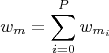 | (1b) |
In (1a), heavily-weighted relationships and nodes with
multiple paths push more of their weight to node m. This
matches user activity as files frequently used together will
receive a higher rank; infrequently seen sequences will
receive a lower rank. The final result list sorts by (1b) from
highest to lowest value.
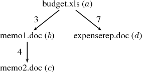
As an example, consider a search for “project budget
requirements” that yields a content-only phase result of
budget.xls with weight wa0 = 1.0. Assume that during the
context-enhancing phase, with parameters P=3, α=0.75 and
no weight cutoff, the relation graph shown in Figure 2 is
loaded from disk. Take node expenserep.doc, abbreviated as
d. The node’s initial weight is wd0 = 0 as it is absent from
the content-only phase results. The algorithm proceeds as
follows for P iterations:
| wd1 | = wa0 ⋅ γ(ead) ⋅ α + (1 - α) γ(ead) ⋅ α + (1 - α)![]](images/usenix075x.png) | | by (1a) | | | |
| | = 1.0 ⋅ (7∕10) ⋅ 0.75 + 0.25 (7∕10) ⋅ 0.75 + 0.25![]](images/usenix077x.png) = 0.775 = 0.775 | | | |
| | wd2 | = 0 | | as wa1=0 | | | |
| | wd3 | = 0 | | as wa2=0 | | | |
| | Finally, the total weight of node d is: | |
| | wd | = 0 + 0.775 + 0 + 0 = 0.775 | | by (1b) | | | | |
The final ordered result list, with terminal weights in
parentheses, is: budget.xls (1.0), expenserep.doc (0.775),
memo1.doc (0.475) and memo2.doc (0.475). In this
example, both memo files have identical terminal weights;
ties are broken arbitrarily.
Though straightforward, this breadth-first reordering and
extension mechanism proves effective [21]. We are also
investigating using machine learning techniques for more
accurately inferring semantic order.
4 Implementation Our implementation runs on Windows NT-based systems.
We use a binary rewriting technique [11] to trace all file
system and interprocess communication calls. We chose such
a user space solution as it allows tracking high-level calls in
the Win32 API.
-
File System Operations
- Opening and closing files (e.g.,
CreateFile, __lopen, __lcreat, CloseHandle); reading
and writing files (e.g., ReadFile,
WriteFile, ReadFileEx, . . . ); moving, copying, and
unlinking files (e.g., MoveFile, CopyFile, DeleteFile,
. . . ).
-
IPC Operations
- Clipboard (DDE), mailslots, named
pipes.
-
Other
- Process creation and destruction: CreateProcess,
ExitProcess.
-
Not interposed
- Sockets, data
copy (i.e., WM_COPYDATA messages), file mapping
(a.k.a. shared memory), Microsoft RPC, COM.
|
| Table 1: | System calls which our tool interposes on. We
trace both the ANSI and Unicode versions of these calls. |
|
When a user first logs in, our implementation instruments
all running processes, interposing on our candidate set
of system calls as listed in Table 1. It also hooks the
CreateProcess call, which will instrument any subsequently
launched executables. Care was required to not falsely trip
anti-spyware tools. Each instrumented process reports its
system call behavior to our background collection daemon,
which uses idle CPU seconds, via the mailslots IPC
mechanism. For performance reasons, each process
amortizes 32K or 30 seconds worth of events across a single
message. The collection daemon contemporaneously creates
two relation graphs: one using temporal locality (§3.1.1) and
one using causality (§3.1.2).
If a file is deleted, its node in the relation graph becomes a
zombie: it relinquishes its name but maintains its current
weight. The basic BFS algorithm uses a zombie’s weight in
its calculations, but a zombie can never be returned in the
search result list. We currently do not prune zombies from
the relation graph.
Content indexing is done using Google Desktop Search
(GDS) with its exposed API. We expect GDS to use
state-of-the-art information retrieval techniques to conduct
its searches. We chose GDS over other content indexing
tools, such as Indri [1], because of its support for more file
types. All queries enter through our interface: only GDS’s
indexing component remains active, its search interface is
turned off. GDS also indexes email and web pages, but we
prune these from the result set. In the future, we intend to
examine email and web work habits and metadata to further
enhance search.
A complication arises, however. GDS allows sorting by
relevance, but it does not expose the actual relevance scores.
These are necessary as they form the initial values of the
basic BFS algorithm (§3.2). We use:
 | (2) |
to seed the initial values of the algorithm. Here, n is the total
number of results for a query, and i is the result’s position in
the result list. Equation (2) is a strict linear progression with relevance values constrained such that the sum of the values
is unity, roughly matching the results one would expect from
a TF/IDF-type system [3]. Soules [20] found that equation
(2)performs nearly as well as real relevance scores: (2)
produces a 10% improvement across all recall levels in
Soules’s study, while real relevance scores produce a 15%
improvement.
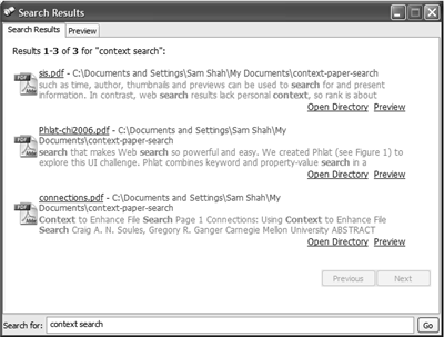
Users interact with our search system through an icon in
the system tray. When conducting a search, a frame, shown
in Figure 3, appears, allowing the user to specify her query
keywords in a small text box. Search results in batches of ten
appear in the upper part of the frame. A snippet of each
search result, if available, is presented, along with options to
preview the item before opening. Previewing is supported by
accessing that file type’s ActiveX control, as is done in web
browsers.
In most desktop search applications, ours included, the
search system is available to users immediately after
installation. Because the content indexer works during idle
time and little to no activity state has been captured to build
our relation graph when first installed, search results during
this initial indexing period are usually quite hapless. We
warn users that during this initial indexing period that their
search results are incomplete.
Our implementation uses a relation window of 30 seconds
and basic BFS with a weight cutoff of 0.1% and parameters
P = 3 and α = 0.75. These parameters were validated by
Soules and Ganger [21].
To prevent excessively long search times, we restrict
the context-enhancing phase to 5 seconds and return
intermediate results from basic BFS. Although, as shown in
our evaluation (§5.3.3), we rarely hit this limit. Due to our
unoptimized implementation, we expect a commercial
implementation to perform slightly better than our results
would suggest.
5 User Study/Evaluation
Our evaluation has four parts: first, we explain the
importance of conducting a user study as our primary
method of evaluation. Second, we describe a controlled trial
coupled with a rating task to assess user satisfaction. The
results indicate that our causality algorithm is indeed an
improvement over content-only indexing, while temporal
locality is statistically indistinguishable. Third, we evaluate
the time and space overheads of our causality algorithm,
finding that both are reasonable. Fourth, we dissect user
elicited feedback of our tool.
5.1 Experimental Approach
Traditional search tools use a corpus of data where queries
are generated and oracle result sets are constructed by
experts [3]. Two metrics, precision (minimizing false
positives) and recall (minimizing false negatives) are then
applied against this oracle set for evaluation. Personal file search systems, however, are extremely
difficult to study in the laboratory for a variety of reasons.
First, as these systems exercise a user’s own content, there is
only one oracle: that particular user. All aspects of the
experiment, including query generation and result set
evaluation, must be completed by the user with their
own files. Second, a user’s search history and corpus is
private. Since the experimenter lacks knowledge of each
user’s data, it’s nearly impossible to create a generic set
of tasks that each user could perform. Third, studying
context-enhanced search is further complicated by the
need to capture a user’s activity state for a significant
length of time, usually a month or more, to develop
our dynamic indices—an impractical feat for an in-lab
experiment.
In lieu of these difficulties with in-lab evaluation,
Soules and Ganger [21] constructed a corpus of data
by tracing six users for a period of six months. At the
conclusion of their study, participants were asked to submit
queries and to form an oracle set of results for those queries.
Since each user must act as an oracle for their system, they
are loathe to examine every file on their machine to build this
oracle. Instead, results from different search techniques were
combined to build a good set of candidates, a technique
known as pooling [3]. Each search system can then be
compared against each oracle set using precision and
recall.
While an excellent initial evaluation, such a scheme may
exhibit observational bias: users will likely alter their
behavior knowing their work habits are being recorded. For
instance, a user may be less inclined to use her system as she
normally would for she may wish to conceal the presence of
some files. It is quite tough to find users who would be
willing to compromise their privacy by sharing their activity
and query history in such a manner.
Further, to generate an oracle set using pooling, we need a
means to navigate the result space beyond that returned from
content-only search. That is, we need to use results from
contextual indexing tools to generate the additional pooled
results. However, the lack of availability of alternative
contextual indexing tools means that pooling may be biased
toward the contextual search tool under evaluation, as
that tool is the only one generating the extra pooled
results.
We also care to evaluate the utility of our tool beyond the
metrics of precision and recall. Precision and recall fail to
gauge the differences in orderings between sets of results.
That is, two identical sets of results presented in different
order will likely be qualitatively very different. Further, while
large gains in mean average precision are detectable to the
user, nominal improvements remain inconclusive [2]. We
would like a more robust measurement that evaluates a user’s
perception of search quality.
For these reasons, we conduct a user study and deploy an
actual tool participants can use. First, we run a pre-post
measures randomized controlled trial to ascertain if users
perceive end-to-end differences between content-only search
and our causality algorithm with basic BFS. Second, we
conduct a repeated measures experiment to qualitatively
measure search quality: we ask users to rate search orderings
of their previously executed queries constructed by
content-only search and of results from our different
dynamic techniques.
5.1.1 Background
We present a terse primer here on the two techniques we
use in our user study. For more information on these
methods, the interested reader should consult Bernard [4] or
Krathwohl [14].
A pre-post measures randomized controlled trial is a study
in which individuals are allocated at random to receive one
of several interventions. One of these interventions is the
standard of comparison, known as the “control,”
the other interventions are referred to as “treatments.”
Measurements are taken at the beginning of the study, the
pre-measure, and at the end, the post-measure. Any change
between the treatments, accounting for the control, can be
inferred as a product of the treatment. In this setup,
the control group handles threats to validity; that any
exhibited change is caused by some other event than the
treatment. For instance, administering a treatment can
produce a psychological effect in the subject where the act
of participation in the study results in the illusion that
the treatment is better. This is known as the placebo
effect.
Consider that we have a new CPU scheduling algorithm
that makes interactive applications feel more responsive
and we wish to gauge any user-perceived difference in
performance against the standard scheduler. To accomplish
this, we segment our population randomly into two groups,
one which uses the standard scheduler, the control group, and
the other receives our improved scheduler, the treatment
group. Neither group knows which one they belong to. At the
beginning of the study, the pre-measure, we ask users to
estimate the responsiveness of their applications with a
questionnaire. It’s traditional to use a Likert scale in which
respondents specify their level of agreement to a given
statement. The number of points on an n-point Likert
scale corresponds to an integer level of measurement,
where 1 to n represents the lowest to highest rating. At
the end of the study, the post-measure, we repeat the
same questionnaire. If the pre- and post-measures in
the treatment group are statistically different than the
pre- and post-measures in the control group, we can
conclude our new scheduler algorithm is rated better by users.
Sometimes it is necessary or useful to take more than one
observation on a subject, either over time or over many
treatments if the treatments can be applied independently.
This is known as a repeated measures experiment. In our
scheduler example, we may wish to first survey our subject,
randomly select an algorithm to use and have the subject run
the algorithm for some time period. We can then survey our
subject again and repeat. In this case, we have more than one
observation on a subject, with each subject acting as its own
control.
Traditionally, one uses ANOVA to test the statistical
significance of hypotheses among two or more means
without increasing the α (false positive) error rate that occurs
with using multiple t-tests. With repeated measures data, care
is required as the residuals aren’t uniform across the
subjects: some subjects will show more variation on some
measurements than on others. Since we generally regard the
subjects in the study as a random sample from the population
at large and we wish to model the variation induced
in the response by these different subjects, we make
the subjects a random effect. An ANOVA model with
both fixed and random effects is called a mixed-effects
model [19].
5.1.2 Randomized Controlled Trial
In our study, we randomly segment the population into a
control group, whose searches return content-only results,
and a treatment group, whose searches return results
reordered and extended by basic BFS using a relation graph
made with the causality algorithm.
To reduce observational bias and protect privacy, our
tool doesn’t track a user’s history, corpus, or queries,
instead reporting aggregate data only. During recruitment,
upon installation, and when performing queries, we
specifically state to users that no personal data is shared
during our experiment. We hope this frees participants to
use their machines normally and issue queries without
hindrance.
The interface of both systems is identical. To prevent
the inefficiency of our unoptimized context-enhancing
implementation from unduly influencing the treatment group,
both groups run our extended search, but the control group
throws away those results and uses content-only results
exclusively.
The experiment is double-blind: neither the participants
nor the researchers knew who belonged to which group. This
was necessary to minimize the observer-expectancy effect;
that unconscious bias on the part of the researchers may
appear during any potential support queries, questions, or
follow ups. The blinding process was computer controlled.
Evaluation is based on pre- and post-measure questionnaires
where participants are asked to report on their behavior using
5-point Likert scale questions. For example, “When I need to
find a file, it is easy for me to do so quickly.” Differences in
the pre- and post-measures against the control group
indicate the overall effect our causality algorithm has
in helping users find their files. We also ask several
additional questions during the pre-survey portion to
understand the demographics of our population and
during the post-survey to elicit user feedback on our
tool.
We pre-test each survey instrument on a small sample of a
half-dozen potential users who are then excluded from
participating in our study. We encourage each pre-tester
to ask questions and utilize “think-alouds,” where the
participant narrates her thought process as she’s taking the
survey. Pre-testing is extremely crucial as it weeds out poorly
worded, ambiguous, or overly technical elements from
surveys. For example, the first iteration of our survey
contained the question, “I often spend a non-trivial amount
of time looking for a file on my computer.” Here, the word
“non-trivial” is not only equivocal, it is confusing. A more
understandable question would be to set an exact time span:
“I often spend 2 minutes or more a day looking for a file on
my computer.”
We also conducted a pilot study with a small purposive
sample of colleagues who have trouble finding their files.
This allowed us to vet our tool and receive feedback on our
study design. Naturally, we exclude these individuals and
this data from our overall study.
5.1.3 Rating Task
We wish to evaluate the n different dynamic algorithms
against each other. Segmenting the study population into n
randomized groups can make finding and managing a large
enough sample difficult. More importantly, as we will show,
controlled experiments on broad measurements for personal
search behavior are statistically indistinguishable between
groups; we believe users have difficultly judging subtle
differences in search systems.
To that end, we also perform a repeated measures
experiment. As we can safely run each algorithm
independently, we contemporaneously construct relation graphs
using both the temporal locality and causality algorithms in
both groups. At the conclusion of the study, we choose up to
k queries at random that were previously successfully
executed by the user and re-execute them. Different views, in
random order, showing each different algorithm’s results are
presented; the user rates each of them independently
using a 5-point Likert scale. We use these ratings to
determine user-perceived differences in each search algorithm.
We define “successfully executed” to be queries where the
user selected at least one result after execution. To prevent
users from rating identical, singular result lists—which
would give us no information—we further limit the list of
successful queries by only considering queries where at least
one pair of algorithms differs in their orderings. With this
additional constraint, we exclude an additional 2 queries
from being rated.
The rating task occurs at the end of the study and not
immediately after a query as we eschew increasing the
cognitive burden users experience when searching. If
users knew they had to perform a task after each search,
they might avoid searches because they anticipate that
additional task. Worse, they might perfunctorily complete
the task if they are busy. In a longer study, it would be
beneficial to perform this rating task at periodic intervals to
prevent a disconnect with the query’s previous intent in the
user’s mind. Previous work has shown a precipitous drop
in a user’s ability to recall computing events after one
month [6].
Finally, we re-execute each query rather than present
results using algorithm state from when the query was first
executed. The user’s contextual state will likely be disparate
between when the query was executed and at the time of the
experiment; any previous results could be invalid and may
potentially cause confusion.
In our experiment, we chose k=7 queries to be rated by
the user. We anecdotally found this to provide a reasonable
number of data points without incurring user fatigue. Four
algorithms were evaluated: content-only, causality, temporal
locality and a “random-ranking” algorithm, which consists
of randomizing the top 20 results of the content-only
method.
5.2 Experimental Results
Our study ran during June and July 2006, starting with
75 participants, all undergraduate or graduate students at the
University of Michigan, recruited from non-computer
science fields. Each participant was required to run our
software for at least 30 days, a period allowing a reasonable
amount of activity to be observed while still maintaining a
low participant attrition rate. Of the initial 75 participants,
27 (36%), consisting of 15 men and 12 women, completed
the full study. This is more than four times the number of
Soules and Ganger [21]. Those who successfully completed
the study received modest compensation.
To prevent cheating, our system tracks its installation,
regularly reporting if it’s operational. We are confident that
we identify users who attempt to run our tool for shorter than
the requisite 30 days. Further, to prevent users from
creating multiple identities, participants must supply their
institutional identification number to be compensated. In
all, we excluded 4 users from the initial 75 because of
cheating.
5.2.1 Randomized Controlled Trial
Evaluating end-to-end effects, as in our controlled trial,
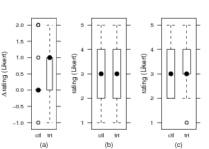
yields inconclusive results. Figure 4 shows box-and-whisker
plots of 5-point Likert ratings for key survey questions
delineated by control and treatment group. For those
unfamiliar: on a box-and-whiskers plot, the median for each
dataset is indicated by the center dot, the first and third
quartiles, the 25th and 75th percentiles respectively—the
middle of the data—are represented by the box. The lines
extending from the box, known as the whisker, represent 1.5
times this interquartile range and any points beyond the
whisker represent outliers. The box-and-whiskers plot is a
convenient method to show not only the location of
responses, but also their variability.
Figure 4(a) is the pre- and post-measures difference on a
Likert rating on search behavior: “When I need to find a
file, it is easy for me to do so quickly.” Sub figures (b)
and (c) are post-survey questions on if the tool would
change their behavior in organizing their files (i.e., “I
would likely put less effort in organizing my files if I
had this tool available”) or whether this tool should be
bundled as part of every machine (i.e., “this tool should
be essential for any computer”). With all measures,
the results are statistically insignificant between the
control and treatment groups (t25 = -0.2876,p=0.776;
t25 = 0.0123,p=0.9903; t25 = -0.4995,p=0.621,
respectively).
We also consider search behavior between the groups.
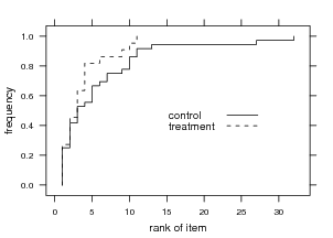
Figure 5 shows the rank of the file selected after performing
a query. Those in the treatment group select items higher in
the list than those in the control group, although not
significantly (t51 = 1.759;p=0.0850).
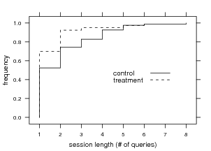
We divide query execution into sessions, each session
representing a series of semantically related queries.
Following Cutrell et al. [5], we define a session to comprise
queries that have an inter-arrival rate of less than 5 minutes.
The session length is the number of queries in a session, or,
alternatively, the query retry rate. As Figure 6 shows, the
treatment group has a shorter average session length
(t97 = 2.136,p=0.042), with geometric mean session lengths
of 1.30 versus 1.66 queries per session, respectively. 13.5%
and 19.0% of sessions in the control and treatment groups,
respectively, ended with a user opening or previewing an
item.
This data is, however, inconclusive. While at first blush it
may appear that with the causality algorithm users are
selecting higher ranked items and performing fewer queries
for the same informational need, it could be just as well
that users give up earlier. That is, perhaps users fail to
select lower ranked items in the treatment group because
those items are irrelevant. Perhaps users in the treatment
group fail to find what they’re looking for and cease
retrying, leading to a shorter session length. In hindsight, it
would have been beneficial to ask users if their query was
successful when the search window was closed. If we had
such data available, we could ascertain whether shorter
session lengths and opening higher ranked items were
a product of finding your data faster or of giving up
faster.
The lack of statistically significant end-to-end effects
stems from the relatively low sample size coupled with the
heterogeneity of our participants. To achieve statistical
significance, our study would require over 300 participants to
afford the standard type II error of β = 0.2 (power t-test,
Δ = 0.2,σ = 0.877,α = 0.05). Attaining such a high
level of replication is prohibitively expensive given our
resources. Instead, our evaluation focuses on our rating
task.
5.2.2 Rating Task
The rating task yielded more conclusive results. 16 out
of our 27 participants rated an aggregate total of 34
queries, an average of 2.13 queries per subject (σ=1.63).
These 34 rated queries likely represent a better candidate
selection of queries due to our “successfully executed”
precondition (§5.1.3): we only ask users to rate queries
where they selected at least one item from the result set for
that search. 11 participants failed to rate any queries: 3 users
failed to issue any, the remaining 8 failed to select at least
one item from one of their searches.
Those remaining 8 issued an average of 1.41 queries
(σ=2.48), well below the sample average of 6.74 queries
(σ=6.91). These likely represent failed searches, but it is
possible that users employ search results in other ways. For
example, the preview of the item might have been sufficient
to solve the user’s information need or the user’s interest may
have been in the file’s path. Of those queries issued
by the remaining 8, users previewed at least one item
17% of the time but never opened the file’s containing
directory through our interface. To confirm our suspicions
about failed search behavior, again it would have been
beneficial to ask users as to whether their search was
successful.
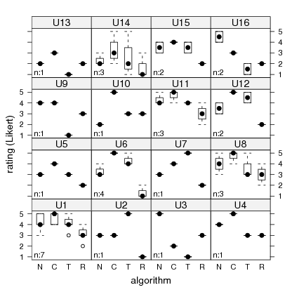
Figure 7 shows a box-and-whiskers plot of each subject’s
ratings for each of the different algorithms. Subjects who
rated no queries are omitted from the plot for brevity. Some
cursory observations across all subjects are that the causality
algorithm usually performs at or above content-only,
with the exception of subjects U3 and U16. Temporal
locality is on par or better than content-only for half of the
subjects, but is rated exceptionally poorly, less than a
2, for a quarter of subjects (U3, U9, U13 and U16).
Surprisingly, while the expectation is for random to be
exceedingly poor, it is often only rated a notch below other
algorithms.
Rigorous evaluation requires care as we have multiple
observations on the same subject for different queries—a
repeated measures experiment. Observations on different
subjects can be treated as independent, but observations on
the same subject cannot. Thus, we develop a mixed-effects
ANOVA model [19] to test the statistical significance of our
hypotheses.
Let yijk denote the rating of the i-th algorithm by the j-th
subject for the k-th query. Our model includes three
categorical predictors: the subject (16 levels), the algorithm
(4 levels), and the queries (34 levels). For the subjects, there
is no particular interest in these individuals; rather, the goal
is to study the person-to-person variability in all persons’
opinions. For each query evaluated by each subject, we wish
to study the query-to-query variability within each subject’s
ratings. The algorithm is a fixed effect (βi), each subject then
is a random effect (ζj) with each query being a nested
random effect (ζjk). Another way to reach the same
conclusion is to note that if the experiment were repeated, thesame four algorithms would be used, since they are part of
the experimental design, but another random sample would
yield a different set of individuals and a different set of
queries executed by those individuals. Our model therefore
is: 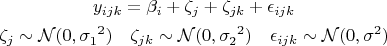 |
(3)
|
| | | 95% Conf. Int.
| | Algorithm | βi | Lower | Upper | p-value† |
|
|
|
|
| | Content only | 3.545 | 3.158 | 3.932 |
| Causality | 4.133 | 3.746 | 4.520 | 0.0042 |
| Temp. locality | 3.368 | 2.982 | 3.755 | 0.3812 |
| Random | 2.280 | 1.893 | 2.667 | <0.0001 |
|
|
|
|
| | σ1 | 0.3829 | 0.1763 | 0.8313 |
| σ2 | 0.4860 | 0.2935 | 0.8046 |
| σ | 0.8149 | 0.7104 | 0.9347 |
| |
†In comparison to content-only.
| Table 2: | Maximum likelihood estimate of the
mixed-effects model given in equation (3). |
|
A maximum likelihood fit of (3) is presented in Table 2.
Each βi represents the mean across the population
for algorithm i. The temporal locality algorithm is
statistically indistinguishable from content-only search
(t99 = -0.880,p=0.3812), while the causality algorithm is
rated, on average, about 17% better (t99 = 2.93,p=0.0042).
Random-ranking is rated about 36% worse on average
(t99 = -6.304,p<0.0001).
Why is temporal locality statistically indistinguishable
from content-only? Based on informal interviews, we purport
the cause of these poor ratings is temporal locality’s
tendency to build relationships that exhibit post-hoc errors:
the fallacy of believing that temporal succession implies a
causal relation.
For example, U16 was a CAD user that only worked on a
handful of files for most of the tracing period (a design she
was working on). The temporal locality algorithm caused
these files to form supernodes in the relation graph; every
other file was related to them. Under results generated by
the temporal locality algorithm, each of her queries
included her CAD files bubbled to the top of the results list.
U9 was mostly working on his dissertation and every
file, as well as some of his music, was lightly related to
each other. The temporal locality algorithm created a
relation graph with 21,376 links with geometric mean
weight of 1.48 (σl=0.688); the causality algorithm,
an order of magnitude fewer, with 1,345 links and a
geometric mean weight of 9.79 (σl=1.512). In his case, it
appears that the temporal algorithm naïvely creates many
lightly-weighted superfluous relations compared with the
causality algorithm.
A user’s work habits will affect the utility of provenance
analysis techniques. Temporal locality’s tendency to
generate large numbers of lightweight false-positive
relationships can be detrimental in many cases, making more
conservative techniques such as causality more broadly
applicable.
The random reordering shares equivalent precision and
recall values as content-only search, but is rated about 35.7%
worse on average. We expect a random ordering to do
phenomenally worse, but hypothesize that personal search
tools are still in their infancy. That is, attention in the
research community has been placed on web search, and
only recently has desktop search become a priority.
There is appreciable room for improvement. It may
also be that users are simply content with having their
desired result on the first page and are apathetic to each
result’s relative ordering within that page. More work is
required to understand a user’s perception of search
orderings.
We further analyze any interactions between other
covariates such as the demographics of participants or user
features (e.g., size of disk, number of files, folder depth). Wefind these covariates either to be statistically insignificant or
to overfit our model.
5.3 Performance
Our results indicate that our causality algorithm increases
user satisfaction of personal file search. However, such a
system is only effective if minimum additional system
resources are required for building, storing, and traversing
the relation graph created by this algorithm. We eschew
discussion of content indexing overheads as these are already
known [16].
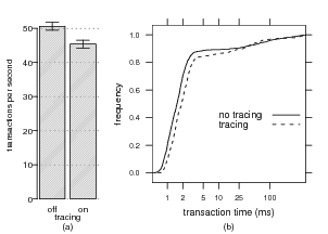
5.3.1 Tracing Performance
We measure the impact building the relation graph has on
foreground performance with the Postmark synthetic
benchmark [13]. Postmark is designed to measure file
system performance in small-file Internet server applications
such as email servers. It creates a large set of continually
changing files, measuring the transaction rates for a
workload of many small reads, writes, and deletes. While not
representative of real user activity in desktop systems,
Postmark represents a particularly harsh setup for our
collection daemon: many read and write events to a
multitude of files inside a single process. Essentially,
Postmark’s workload creates a densely-connected relation
graph.
We run 5 trials of Postmark, with and without tracing, with
50,000 transactions and 10,000 simultaneous files on an IBM
Thinkpad X24 laptop with a 1.13 GHz Pentium III-M CPU
and 640 MB of RAM, a modest machine by today’s
standards. The results are shown in Figure 8(a). Under
tracing, Postmark runs between 7.0% and 13.6% slower
(95% conf. int.; t8=7.211,p<0.001). Figure 8(b) shows a
c.d.f. of Postmark’s transaction times with and without
tracing across a single run. There is a relatively constant
attenuation under tracing, which reflects the IPC overhead of
our collection daemon and the additional disk utilization due
to relation graph updates. This additional slowdown caused
by relation graph construction is in line with other Win32
tracing and logging systems [15].
5.3.2 Space Requirements
We examine the additional space required by our relation
graphs. During the user study, the tool logged the size of
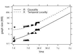
each relation graph every 15 minutes. Figure 9 shows
relation graph growth over time for the heaviest user
in our sample, U3. Each relation graph grows linearly
(r2 = 0.861 and r2 = 0.881 for causality and temporal
locality, respectively). While the worst case graph growth is
O(F2), where F is the number of files on a user’s system,
these graphs are generally very spare: most files only
have relationships to a handful of other files as a user’s
working set at any given time is very small. In one year, we
expect the causality relation graph for U3 to grow to
about 44 MB; in five years, 220 MB. This is paltry
compared to the size of modern disks and represents an
exceedingly small fraction of the user’s working set.
These results suggest that relation graph size isn’t an
obstacle.
5.3.3 Search Performance
The time to answer a query must be within reasonable
bounds for users to find the system usable. In our
implementation (§4), we bound the context-enhancing phase
to a maximum of 5 seconds.
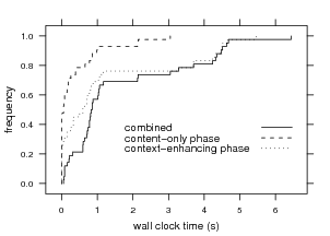
For every query issued during the user study, we log
the elapsed wall clock time in the content-only and
context-enhancing phases. Figure 10 shows these results.
Half of all queries are answered within 0.8 seconds,
three-quarters within 2.8 seconds, but there is a heavy tail.
The context-enhancing phase takes about 67% of the entire
search process on average. We believe these current search
times are within acceptable limits.
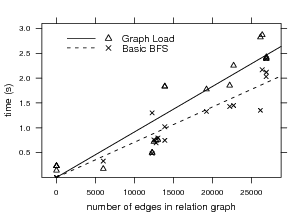
Recall that the context-enhancing phase consists of two
distinct subphases: first, the loading of the relation graph,
followed by execution of the basic BFS algorithm (§3.2). To
understand the performance impact of these subphases,
previous queries issued by the author were re-executed, for 5
trials each under a cold cache, with the relation graph from a
6-month trace. Figure 11 shows the time spent for each
query based on the number of edges from the relation graph
loaded for that query. For non-empty graphs, loading the
relation graph took, on average, between 3.6% and 49.9%
longer (95% conf. int.) than the basic BFS subphase (paired
t15 = -2.470,p=0.026).
Both loading the relation graph and basic BFS execution
support linear increase models (r2 = 0.948 and r2 = 0.937,
respectively). This is apparent as each subphase requires both
Ω(F2) space and time, where F is the number of files on a
user’s system. As these are lower bounds, the only way to
save space and time would be to ignore some relationships. If
we could predict a priori which relationships were most
relevant, we could calculate, at the expense of accuracy,
equation (1a) for those pairs. Further, we could cluster those
relevant nodes together on disk, minimizing disk I/Os during
graph reads.
5.4 User Feedback
| Question | μ | σ |
|
|
| | I would prefer an interface that shows more information. | 3.84 | 1.34 |
| I find it easy to think of the correct search keywords. | 3.69 | 0.85 |
| I would prefer if I could look over all my machines. | 3.46 | 1.39 |
| This tool should be essential for any computer. | 3.30 | 1.25 |
| I like the interface. | 3.15 | 1.40 |
|
|
| | I would prefer if my email and web pages are included in the search results. | 3.00 | 1.58 |
| I would likely put less effort in organizing my files if I had this tool available. | 2.92 | 1.12 |
| |
| Table 3: | Additional 5-point Likert ratings asked
of treatment group users at the end of the study
period (N = 13). |
|
During the post-survey phase of our study, our questionnaire
contained additional 5-point Likert ratings. A tabulation of
subject’s responses for the treatment group are shown in
Table 3. While it’s difficult to draw concrete answers due to
the high standard deviations, we can develop some general
observations.
An area for improvement is the user interface. Our
results are presented in a list view (Figure 3), but using
more advanced search interfaces, such as Phlat [5],
that allow filtering through contextual cues may be more
useful. Different presentations, particularly timeline
visualizations, such as in Lifestreams [9], may better
harness users’ memory for their content. There is
a relatively strong positive correlation (ρ = 0.698) between
liking the interface and finding the tool essential; a better
interface will likely make the tool more palatable for
users.
Based on informal interviews, we found that participants
used our search tool as an auxiliary method of finding
content: they first look through their directory hierarchy for a
particular file, switching to keyword search after a few
moments of failed hunting. Participants neglect to use our
search tool as a first-class mechanism for finding content. A
system that is integrated into the OS, including availability
from within application “open” dialogs, may cause a
shift in user’s attitudes toward using search to find their
files.
We found it surprising that users wished to exclude email
and web pages from their search results; two-thirds of users
rate this question a three or below. Our consultations reveal
that many of these users dislike a homogeneous list of
dissimilar repositories and would rather prefer the ability to
specify which repository their information need resides
in. That is, a user knows if they’re searching for a file,
email or web page, let them easily specify which. We
needn’t focus on mechanisms to aggregate heterogeneous
forms of context spread across different repositories
into a unifying search result list, but to simply provide
an easy mechanism to refine our search to a specific
repository.
6 Personal Search Behavior
Finally, we explore the search behavior of our sample
population. Recall that, for privacy reasons, we do not log
any information about the content of users’ indices or search
results.
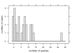
Our population issued 182 queries; the distribution
per user is shown in Figure 12. The average number
of queries issued per user is 6.74 (σ=6.91). Most
queries, 91%, were fresh, having never been issued
before. About 9% of search terms were for filenames.
Since Windows XP lacks a rapid search-by-filename
tool similar to UNIX’s slocate, users were employing
our tool to find the location of files they already knew
the name of. Most queries were very short, averaging
1.16 words (σ=0.462), slightly shorter than the 1.60
and 1.59 words reported for Phlat [5] and SIS [8]
respectively.
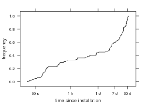
Figure 13 shows when queries are issued after installation.
A sizable portion of queries are issued relatively soon
after installation as users are playing with the tool. Even
though we warn users that search results are initially
incomplete because the content indexer has not built enough
state and the relation graph is sparse (§4), it may be
prudent to disallow searching until a reasonable index
has been built as not to create an unfavorable initial
impression.
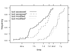
Figure 14 shows the last access time and last modification
times of items opened after searching. The starred versions
represent last access and modification times of queries issued
at least a day after installation. During the first day,
users might be testing the tool against recent work and,
hence, recently accessed files. Anecdotal evidence of this
effect can be observed by the shifted last accessed curve.
After the warm-up period, half of all files selected were
accessed within the past 2 days. It appears users are
employing our tool to search for more than archival
data.
7 Conclusions & Future Work
By measuring users perception of search quality with our
rating task (§5.2.2), we were able to show that using
causality (§3.1.2) as the dynamic re-indexing component
increases user satisfaction in search, being rated 17% higher
than content-only indexing or temporal locality, on average
over all queries. While our contextual search mechanism
lacked any significant increases in end-to-end effects in our
randomized controlled trial (§5.2.1), this stemmed from an
insufficiently large sample size. It is prohibitively expensive
to secure such high levels of replication, making our rating
task a more appropriate methodology for evaluating personal
search systems. These results validate that using the
provenance of files to reorder and extend search results is an
important complement to content-only indexing for personal
file search.
There is still considerable future work in this area. While
we find temporal locality (§3.1.1) infelicitous in building a
contextual index, one should not dismiss temporal bounds
altogether. We are investigating using window focus
and input flows in delineating tasks to create temporal
boundaries.
Further, our tool only has limited access: a user’s
local file system. We could leverage electronic mail,
their other devices and machines, and distributed file
systems, stitching context from these stores together to
provide further benefit. Since these indices may span the
boundaries of multiple machines and administrative
domains, we must be careful to maintain user privacy
and access rights. We are investigating these and other
avenues.
Finally, the tradition in the OS community, and we have
been as guilty of this as any, has been to evaluate systems on
a small number of users—usually departmental colleagues
known to the study author. These users are generally
recognized as atypical of the computing population at large:
they are expert users. As the community turns its attention
away from performance and toward issues of usability and
manageability, we hope our work inspires the OS communityto consider evaluating their systems using the rigorous
techniques that have been vetted by other disciplines. User
studies allow us to determine if systems designed and
tested inside the laboratory are indeed applicable as we
believe.
Acknowledgements
We’d like to thank Mark Ackerman for his help with our user
study. This research was supported in part by the National
Science Foundation under grant number CNS-0509089. Any
opinions, findings, and conclusions or recommendations
expressed in this paper are those of the authors and do not
necessarily reflect the views of the National Science
Foundation.
References
[1] Nasreen
Abdul-Jaleel, James Allan, W. Bruce Croft, Fernando Diaz, Leah
Larkey, Xiaoyan Li, Donald Metzler, Mark D. Smucker, Trevor
Strohman, Howard Turtle, and Courtney Wade. UMass at TREC
2004: Notebook. In TREC 2004, pages 657–670, 2004.
[2] James Allan, Ben Carterette, and Joshua Lewis. When will
information retrieval be “good enough”? In SIGIR 2005, pages
433–440, Salvador, Brazil, 2005.
[3] Ricardo Baeza-Yates and Berthier Ribeiro-Neto. Modern
Information Retrieval. ACM Press, New York, 1999.
[4] H. Russell Bernard. Social Research Methods. Sage
Publications Inc., 2000.
[5] Edward Cutrell, Daniel C. Robbins, Susan T. Dumais, and
Raman Sarin. Fast, flexible filtering with Phlat—personal search
and organization made easy. In CHI 2006, pages 261–270,
Montréal, Québec, Canada, 2006.
[6] Mary Czerwinski and Eric Horvitz. An investigation of
memory for daily computing events. In HCI 2002, pages
230–245, London, England, 2002.
[7] John R. Douceur and William J. Bolosky. A large-scale
study of file-system contents. In IMC 1999, pages 59–70, 1999.
[8] Susan T. Dumais, Edward Cutrell, J. J. Cadiz, Gavin Jancke,
Raman Sarin, and Daniel C. Robbins. Stuff I’ve Seen: A system
for personal information retrieval and re-use. In SIGIR 2003,
pages 72–79, Toronto, Ontario, Canada, 2003.
[9] Scott Fertig, Eric Freeman, and David Gelernter. Lifestreams:
An alternative to the desktop metaphor. In CHI 1996, pages
410–411, Vancouver, British Columbia, Canada, April 1996.
[10] David K. Gifford, Pierre Jouvelot, Mark A. Sheldon, and
James W. O’Toole. Semantic file systems. In SOSP 1991, pages
16–25, Pacific Grove, CA, October 1991.
[11] Galen Hunt and Doug Brubacher. Detours: Binary
interception of Win32 functions. In 3rd USENIX Windows NT
Symposium, pages 135–143, Seattle, WA, USA, 1999.
[12] David Huynh, David R. Karger, and Dennis Quan. Haystack:
A platform for creating, organizing and visualing information
using RDF. In Semantic Web Workshop, 2002.
[13] Jeffrey Katcher. Postmark: A new filesystem benchmark.
Technical Report 3022, Network Appliance, October 1997.
[14] David R. Krathwohl. Methods of Educational and Social
Science Research: An Integrated Approach. Waveland Inc., 2nd
edition, 2004.
[15] Jacob R. Lorch and Alan Jay Smith. The VTrace tool:
building a system tracer for Windows NT and Windows 2000.
MSDN Magazine, 15(10):86–102, October 2000.
[16] Donald Metzler, Trevor Strohman, Howard Turtle, and
W. Bruce Croft. Indri at TREC 2004: Terabyte Track. In TREC
2004, 2004.
[17] Kiran-Kumar Muniswamy-Reddy, David A. Holland, Uri
Braun, and Margo Seltzer. Provenace-aware storage systems. In
USENIX 2006, pages 43–56, Boston, MA, USA, 2006.
[18] Nuria Oliver, Greg Smith, Chintan Thakkar, and Arun C.
Surendran. SWISH: Semantic analysis of window titles and
switching history. In IUI 2006, pages 194–201, Sydney,
Australia, 2006.
[19] José C. Pinheiro and Douglas M. Bates. Mixed-Effects
Models in S and S-Plus. Springer, New York, 2000.
[20] Craig A. N. Soules. Using context to assist in personal file
retrieval. PhD thesis, Carnegie Mellon University, 2006.
[21] Craig A. N. Soules and Gregory R. Ganger. Connections:
using context to enhance file search. In SOSP 2005, pages
119–132, Brighton, UK, 2005.
[22] Jaime Teevan, Christine Alvarado, Mark S. Ackerman, and
David R. Karger. The perfect search engine is not enough: a
study of orienteering behavior in directed search. In CHI 2004,
pages 415–422, 2004.
|