Probabilistic Inference in Queueing Networks
Charles Sutton |
Although queueing models have long been used to model the performance of computer systems, they are out of favor with practitioners, because they have a reputation for requiring unrealistic distributional assumptions. In fact, these distributional assumptions are used mainly to facilitate analytic approximations such as asymptotics and large-deviations bounds. In this paper, we analyze queueing networks from the probabilistic modeling perspective, applying inference methods from graphical models that afford significantly more modeling flexibility. In particular, we present a Gibbs sampler and stochastic EM algorithm for networks of M/M/1 FIFO queues. As an application of this technique, we localize performance problems in distributed systems from incomplete system trace data. On both synthetic networks and an actual distributed Web application, the model accurately recovers the system’s service time using 1% of the available trace data.
Performance models of computer systems have the potential to address a wide variety of problems, including capacity planning, resource allocation, performance tuning, anomaly detection, and diagnosis of performance bugs. A well-studied class of performance model is that of queueing models. Queueing models predict the explosion in system latency under high workload in a way that is often reasonable for real systems, allowing the model to extrapolate from performance under low load to performance under high load. This is useful because it allows us to predict the amount of load that will cause a system to become unresponsive, without actually allowing it to fail. Despite these advantages, practitioners seldom use queueing theory, or performance models of any kind, to analyze large-scale commercial computer systems. A main reason for this is that queueing theory has a reputation among computing practitioners for making unrealistic assumptions on the distributions over system response times, and of lacking robustness to divergence from the modeling assumptions [5].
In addition, many important statistical questions about system performance are difficult to answer using queueing theory. One example is diagnosis of past performance problems, for example: “Five minutes ago, a brief spike in workload occurred. Which parts of the system were the bottleneck during that spike?” This is a different question from asking about a hypothetical future workload; essentially, it is a “What happened?” question rather than a “What if?” question. A second type of question is diagnosis of slow requests: “During the execution of the 1% of requests that perform poorly, which system components receive the most load?” The bottleneck for slow requests could be very different than the bottleneck for average requests, for example, if a storage or network resource is failing intermittently. This also demonstrates another type of performance localization, which is that poor performance of any component can be due to intrinsic performance or due to heavy load.
A key point of this paper is that both types of difficulties—unrealistic distributional assumptions and limited ability to answer statistical questions—arise not from queueing models themselves, but from the way in which they are analyzed. Because of their rich structure, queueing models are notoriously difficult, and even the simplest models, such as M/M/1 queues, require approximations. Classically the approximations are performed in one of two ways: either by computing the steady-state response time distribution (or its moments such as the mean), or by bounding the response times using the theory of large deviations. Although these approximations provide important insights into a large class of models, they have several practical limitations. First, they are often difficult to calculate for realistic distributions, and unrealistic assumptions can lead to inaccurate predictions. Second, even if the steady-state distribution can be computed exactly, it often does not directly answer statistical questions of interest: the steady-state distribution is an exact solution to an approximate problem. For example, even total knowledge of the steady-state distribution does not help answer the modeling questions presented above.
The main contribution of this paper is to propose a new family of analysis techniques for queueing models, based on a statistical viewpoint. The main idea is to measure from the running system both the total number of requests, and a small set of actual arrival and departure times. Then, rather than analyzing the steady-state distribution, we analyze the conditional distribution over the arrival and departure times that were not measured, conditioned on the small set of observations. In statistics, this distribution is called a posterior distribution, because it is obtained after observing data.
Even for simple models, representing the posterior distribution is intractable. To handle this, we view a queueing network model as a structured probabilistic model, a perspective that essentially combines queueing networks and graphical models. This novel viewpoint allows us to apply modern approximate inference techniques from the probabilistic reasoning and machine learning communities, such as Markov chain Monte Carlo methods that sample from the posterior distribution.
As an illustration of this approach, in this paper we derive a Gibbs sampler (Section 3) and a stochastic EM algorithm (Section 4) for networks of M/M/1 queues. This allows us to estimate the parameters of a queueing network from an incomplete sample of arrival and departure times. On both synthetic data (Section 5.1) and performance data measured from a simple Web application (Section 5.2), we estimate the mean service and waiting time of each queue, with accuracy sufficient to perform localization, from 1% of the available data.
Despite the long history of queueing models and queuing networks, we are unaware of any existing work that treats them as latent-variable probabilistic models, and attempts to approximate the posterior distribution directly. Furthermore, we are unaware of any technique for estimating the parameters of a queueing model from an incomplete sample of arrivals and departures.
In this section, we describe queueing networks from the probabilistic modeling perspective. As an example, consider a single-processor FIFO queue. This is a system that can process one request at time and has a queue to hold incoming requests. Requests arrive at the queue according to times drawn from some stochastic process, such as a Poisson process. Requests are removed from the queue in a first-in first-out (FIFO) manner. The amount of time a request spends in the queue is called the waiting time w. Once the request leaves the queue, it begins processing, and remains in service for some service time s. All service times are drawn independently from some distribution, such as an exponential distribution with rate µ. The total response time is defined as r := s + w. In this way, the model decomposes the total response time into two components: the waiting time, which represents the effect of system load, and the service time, which is independent of system load. From this perspective, an attraction of queueing models is that they specify the distribution over waiting times as a function of the distributions over arrival and service times.
Many systems are naturally modeled as a network of queues. For example, web services are often designed in a “three tier” architecture, in which the first tier is a presentation layer that generates the response HTML, the second tier performs application-specific logic, and the third tier handles persistent storage, often using a relational database. Each tier is replicated on redundant servers, so it is natural to use one queue for each redundant server on each tier and one queue for the network connection between them. Such a queueing network is depicted in Figure 1. As another example, a distributed storage system might use one queue for each storage server, and one queue for each disk. Finally, single systems can be modeled using a network with one queue for the CPU, one for each disk, one for the memory, etc.
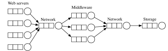
Figure 1: A queueing network model of a three-tier web service. The circles indicate servers, and the boxes indicate queues.
We model the process of a task through the system as a probabilistic finite state machine. After each transition, the FSM emits the next queue for the task. The task arrives at that queue, waits in queue for some time w, receives service for some time s, and then samples a new FSM state. The task is completed when it enters the final state of the FSM. We expect that the system FSM is defined in advance, for example, from a known protocol or multi-tier network application. We denote so that the transition distribution between sates as p(σ′ | σ), and the emission distribution over queues q is p(q | σ).
A series of tasks can be represented compactly by the notion of an event. An event represents the process of a task arriving at a queue, waiting in queue, receiving service, and departing. Each state transition corresponds to an event e = ( ke, σe, qe, ae, de ), where ke is the task that changed state, σe is the new state, qe the new queue, ae the arrival time, and de the departure time. Every event e has two predecessors: a within-queue predecessor ρ(e), which is generated by the previous task to arrive at queue qe, and a within-task predecessor π(e), which is generated by the task’s previous arrival.
Notice that the service time se can be computed deterministically from the set of all arrivals and departures. Finally, arrivals to the system as a whole are represented using special initial events, which arrive at a designated initial queue q0 at time 0 and depart at the time that the task entered the system. This convention simplifies the notation considerably, because now the interarrival time distribution is simply the service distribution for q0.
Now we are able to write down the joint distribution for a set of events E processed by the system. This is
| p(E) = |
| 1{ae = dπ(e)} 1{de = se + max ae, dρ(e) } |
(1) Many choices are possible for the service time distributions. As an illustration of the modeling technique, in this paper we focus on M/M/1 queues, so that the service time for each queue q is exponential with rate µq, and the interarrival time exponential with rate λ = µq0. However, this viewpoint is just as useful for more general service distributions, and we are currently generalizing the sampler to that case.
In this section, we tackle the challenging task of developing a Gibbs sampler for a M/M/1/FIFO queueing network. The data is a set of events E = { ( ke, qe, σe, ae, de)} describing a set of tasks processed by the system. Suppose that we measure the arrival times from a subset of events O ⊂ E. Then a probabilistic model, such a queueing model, allows us to make inferences about the unobserved events via the posterior distribution p(E|O). Because this is a complex distribution over a high-dimensional continuous space, we cannot compute it exactly, so instead we sample from the distribution, using a procedure called Gibbs sampling.
The sampler is complicated by two issues that are specific to queueing models. The first is that we observe only arrival and departure times, not service times directly. Whereas any combination of service times corresponds to a valid event set, the arrival and departure times have several deterministic dependencies, namely that ae = dπ(e) and de = se + max ae,dρ(e) , which must be respected by the sampler. Deterministic dependencies like this are known to impair the performance of Gibbs samplers, so to address this we must design the sampler and its initialization carefully. The second complication is that changing one departure time de can affect the departures of arbitrarily many later events, because no other job can be serviced while de is in queue. This means that the Markov blanket for a single departure can be very large.
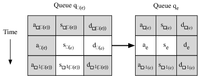
Because of the deterministic dependencies mentioned above, when resampling ae, we must also resample dπ(e), se, sπ(e), and sρ−1(π(e)). The notation E\ e means all of the information from E, except for those five variables. These variables are illustrated in Figure 2. To address the issue of deterministic constraints, we make two other assumptions. First, we assume the FSM paths (σe, qe) for all events are known. If these paths are unknown for some events, they can be resampled by an outer Metropolis-Hastings step. Second, when resampling an arrival time, we hold fixed the order of arrivals at each queue. This is essentially equivalent to assuming that, between every two observed events, we know how many unobserved events occurred. This is easy to measure in actual systems, by maintaining an event counter that is transmitted only when an event is observed. This assumption is useful because it means that resampling a departure de can affect the service time only of the next event dρ−1(e), rather than every subsequent event in qe.
Now, the conditional distribution over the arrival ae contains terms that reflect the service time se of the resampled event, the service time sπ(e) of the within-task predecessor, and the service time sρ−1(π(e)) of the next event in the earlier queue. The distribution to be sampled is p(ae | E\ e), which we write as p(ae | E\ e) = Z−1 g(ae), where g(ae) is
|
Because the arrival order is fixed, and the queues are FIFO, there are several deterministic constraints on ae. These are that ae must be greater than L = max{aπ(e), dρ(π(e)), aρ(e)} and less than U = min{de, aρ−1(e), dρ−1(π(e)) }.
The normalizing constant Z can be computed by integrating both sides of (2), but computing the required integral is complicated by the two maximizations that involve ae. To handle this, divide the integral defining Z into three parts, which are bounded by the next arrival aρ−1(π(e)) at the earlier queue and the previous departure dρ(e) at the later queue. Since those can occur in either order, the boundaries of the integration are A = min{ aρ−1(π(e)), dρ(e)} and B = max{ aρ−1(π(e)), dρ(e)}. Then we write Z = Z1 + Z2 + Z3, where Z1 is restricted to (L,A), Z2 to (A,B). and Z3 to (B,U). Each of these smaller integrals can be solved analytically, because the maximization within g(ae) vanishes. Also, each integral has a natural interpretation: Z1 / Z is the probability that ae falls in the interval (L, A); Z2 / Z the probability for (A,B), and Z3/Z the probability for (B,U). With this normalizing constant Z, we can sample from (2) by taking the inverse cdf of each case. This yields the sampler described in Figure 3.
- Sample V ∼ Unif 0 ; 1 .
- Compute
where
ae =
⎧
⎪
⎪
⎨
⎪
⎪
⎩
−µπ(e)−1 log ⎛
⎝exp{−µπ(e)L} + V
exp{−µπ(e)A} − exp{−µπ(e) L}
⎞
⎠with probability Z1 / Z A2 with probability Z2 / Z
µe−1 log ⎛
⎝exp{µeB} + V exp{µeU} − exp{µe B} ⎞
⎠with probability Z3 / Z (3) and TrExp(µ; N) denotes the exponential distribution with rate µ truncated to the interval (0,N).
A2 ∼
⎧
⎪
⎨
⎪
⎩
Unif A ; B if dρ(e) ≥ aρ−1(π(e)) Unif A ; B if dρ(e) < aρ−1(π(e)) and δµ = 0 A + TrExp(| δµ |; B−A) if dρ(e) < aρ−1(π(e)) and δµ > 0 B − TrExp(| δµ |; B−A) if dρ(e) < aρ−1(π(e)) and δµ < 0 . (4)
Figure 3: Sampler for the local conditional distribution required by the Gibbs sampler.
Finally, initializing the Gibbs sampler requires finding arrival times for the unobserved events that are feasible with respect to the deterministic constraints described above. Initialization is further complicated because a task may contain both observed and unobserved arrivals, so an arrival may be constrained both by its queue and its task. To handle this, given an initial setting µ of the mean service times, we use a linear program to minimize ∑e | se − µqe | subject to the deterministic constraints.
From a sample of events O ⊂ E, we may wish to obtain a point estimate µq of the mean service time of each queue q and the arrival rate λ. A natural method is EM, but the E-step cannot be performed exactly. The E-step can be approximated using the output of a Gibbs sampler, which results in Monte Carlo EM [7], but this requires running an independent Gibbs sampler for a large number of iterations at each outer EM iteration. Instead, we use stochastic EM (StEM), in which the E-step consists of replacing the unobserved arrivals with the output of only one iteration of a Gibbs sampler [2, 4, 3]. The M-step is the standard maximum likelihood estimator for λ and { µq }. Once a point estimate µ of the mean service times available, an estimate of the waiting time can be obtained by running the Gibbs sampler with µ fixed.
In this section, we demonstrate the performance of the model on the task of localizing performance faults in distributed systems from incomplete arrivals. The goal is to localize performance problems to one component of the system, and to report whether the large response time is due to the intrinsic performance of the system, or simply due to increased load. This problem can be cast as one of estimating the service time and waiting time for each queue in a queueing network. For example, if the mean waiting time at the database queue is disproportionately large, then we conclude the database is the bottleneck for that time period. If the response times for all requests are observed, then this task is trivial, but this level of instrumentation can have an unacceptable computational cost. For example, in a performance study of the Coral distributed web cache, recording the trace data for all requests would require 123 GB per day (uncompressed).1 This is why we assume that arrival times and rates are measured for only a subset of requests.
First we evaluate the accuracy of the Gibbs sampler and StEM procedure in simulation. Because the shape of the distribution over arrivals depends on the system load, we evaluate both lightly loaded and heavily loaded systems. We sample arrivals and departures from a number of three-tier queueing networks, as depicted in Figure 1, but without the network queues. In all cases the arrival rate was set to λ = 10.0 and all of the service rates to µ = 5.0. These parameters where chosen so that a tier with a single server is heavily overloaded, one with two servers barely overloaded, and one with four servers moderately loaded. We generate synthetic data from five different network structures, with differing numbers of queues at each tier, in order to vary the system bottleneck. From each structure, we generate 1000 tasks and observe all arrivals for a random sample of tasks. Then we estimate the waiting and service time of each queue using the Gibbs sampler and StEM. For each network structure, we repeat this procedure 10 times.
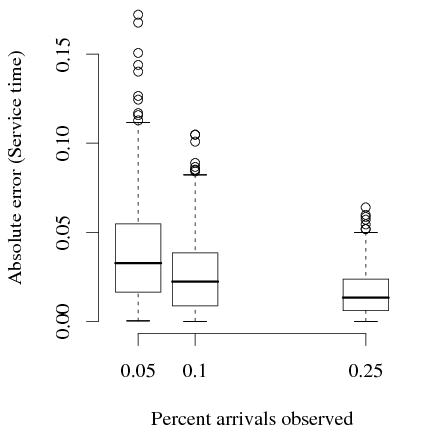
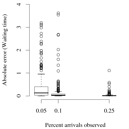
Figure 4 shows the accuracy in the recovered service times and waiting times as a function of the percentage of arrivals that are observed. Each point is the absolute error in the estimate for one queue in one repetition for one simulated structure. Even with a small amount of data, the accuracy is sufficient for localizing performance problems. With 5% of tasks observed, the median absolute error in service time is 0.033 and for waiting time 1.35. For queues that are overloaded, the waiting time tends to be an order of magnitude greater than the service time, so it is not surprising that the error is larger.
Traditional queueing theory does not provide a method for estimating the service times given an incomplete sample of response times. As a baseline, we use the sample mean of the service time for the tasks that are observed. This comparison is unfair to StEM, because the baseline uses the true service times from the observed tasks, information that is not available to StEM. Comparing these estimators, although the mean error is almost identical, StEM has only two-thirds of the variance (StEM variance: 9.09 × 10⁻⁴, Mean-observed-service variance: 1.37 × 10⁻³ ).
Now we evaluate the queueing model on data generated by instrumenting a simple benchmark Web application. The system is a Web application for voting on movies, written using the Ruby on Rails application framework. This data was previously used in [1]. Almost all of the page content is dynamically generated. We run ten identical instances of the web server process, which computes the dynamic content, on a single machine. A separate machine runs a MySQL database for persistent storage. The software load balancer haproxy is used to handle incoming requests, which allows us to estimate the network transmission time of the HTTP request and response.
To model this system as a queueing network, we use one queue for each of the 10 web server instances, one for the database, and one for the network transmission time to and from the system. We generate 5759 requests to the system using an automatic workload generator, increasing the load linearly over 30 min. This results in 23036 total arrival events in the queueing model. The running time of the StEM/Gibbs procedure is difficult to quantify theoretically, because it depends on the number of iterations required to reach convergence. However, the sampler scales primarily in the number of unobserved arrival events, not in the number of servers.
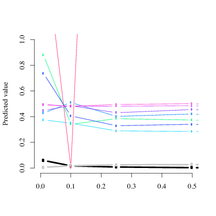
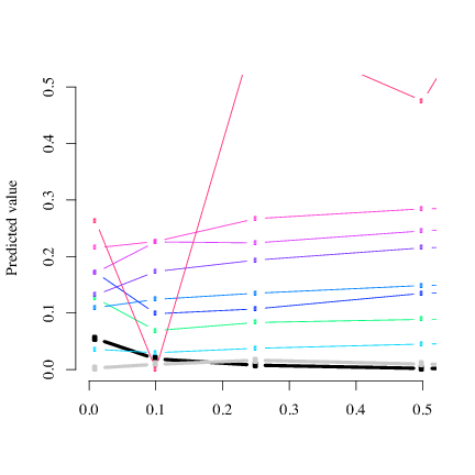
The parameter estimates from various amounts of observed traces are shown in Figure 5. In this figure, the thick black line represents the estimates for the network queue, the thick gray line the database queue, and the thin lines the 10 web servers. If 100% of the data is observed, the estimates are essentially the same as for 50% observed data. In addition, the estimates are stable as the amount of data decreases, producing reasonable estimates even with 10% of the observed data.
One of the queues in the Figure 5 is a clear exception. This is because the load balancer assigned an unusually small number of requests (19) to that server during the observed time period. With such a small amount of data, estimation can be expected to be unstable.
Queueing models have been long studied in telecommunications, operations research, and performance modeling of computer networks and systems. There has been recent interest in modeling dynamic Web services by queueing networks [6, 8]. There is also recent work using queueing models to initialize more flexible models, namely regression trees [5].
In this paper, we have introduced a new class of techniques for analyzing queueing models by approximating the posterior distribution directly using modern approximate inference algorithms from graphical models. We are aware of no previous work applying inference algorithms from graphical models to networks of queues. On both synthetic and real-world data, we have shown that this perspective allows parameter estimation from incomplete data. Perhaps the most useful aspect of this perspective, however, is the flexibility that it affords for future modeling work, including more general arrival and service distributions, model selection, and online, distributed inference.
We thank Peter Bodik for providing the data used in Section 5.2, and George Porter, Rodrigo Fonseca, and Randy Katz for helpful conversations. The movie voting application was developed primarily by Michael Armbrust and Jacob Abernethy. This research is supported in part by gifts from Sun Microsystems, Google, Microsoft, Cisco Systems, Fujitsu America, Hewlett-Packard, IBM, Network Appliance, Oracle, Siemens AB, and VMWare, and by matching funds from the State of California’s MICRO program (grants 06-152, 07-010, 06-148, 07-012, 06-146, 07-009, 06-147, 07-013, 06-149, 06-150, and 07-008), the National Science Foundation (grant #CNS-0509559), and the University of California Industry/University Cooperative Research Program (UC Discovery) grants COM06-10213 and COM07-10240.
This document was translated from LATEX by HEVEA.