
Scalable system monitoring is a fundamental abstraction for large-scale networked systems. It enables operators and end-users to characterize system behavior, from identifying normal conditions to detecting unexpected or undesirable events--attacks, configuration mistakes, security vulnerabilities, CPU overload, or memory leaks--before serious harm is done. Therefore, it is a critical part of infrastructures ranging from network monitoring [30,32,10,23,54], financial applications [3], resource scheduling [27,53], efficient multicast [51], sensor networks [25,27,53], storage systems [50], and bandwidth provisioning [15], that potentially track thousands or millions of dynamic attributes (e.g., per-flow or per-object state) spanning thousands of nodes.
Three techniques are important for scalability in monitoring systems: (1)
hierarchical
aggregation [51,30,53,27]
allows a node to access detailed views of nearby information and
summary views of global information, (2) arithmetic
filtering [30,31,36,42,56]
caches recent reports and only transmits new information if it differs
by some numeric threshold
(e.g., ![]() 10%) from the cached report, and (3) temporal
batching [32,36,42,51]
combines multiple updates that arrive near one another in time into a
single message.
Each of these techniques can reduce monitoring
overheads by an order of magnitude or
more [30,31,53,42].
10%) from the cached report, and (3) temporal
batching [32,36,42,51]
combines multiple updates that arrive near one another in time into a
single message.
Each of these techniques can reduce monitoring
overheads by an order of magnitude or
more [30,31,53,42].
As important as these techniques are for scalability, they interact badly with node and network failures: a monitoring system that uses any of these techniques risks reporting highly inaccurate results.
These effects can be significant. For example, in an 18-hour interval for a PlanetLab monitoring application, we observed that more than half of all reports differed from the ground truth at the inputs by more than 30%. These best effort results are clearly unacceptable for many applications.
To address these challenges, we introduce Network Imprecision (NI), a new consistency metric suitable for large-scale monitoring systems with unreliable nodes or networks. Intuitively, NI represents a ``stability flag'' indicating whether the underlying network is stable or not. More specifically, with each query result, NI provides (1) the number of nodes whose recent updates may not be reflected in the current answer, (2) the number of nodes whose inputs may be double counted due to overlay reconfiguration, and (3) the total number of nodes in the system. A query result with no unreachable or double counted nodes is guaranteed to reflect reality, but an answer with many of either indicates a low system confidence in that query result--the network is unstable, hence the result should not be trusted.
We argue that NI's introspection on overlay state is the right abstraction for a monitoring system to provide to monitoring applications. On one hand, traditional data consistency algorithms [56] must block reads or updates during partitions to enforce limits on inconsistency [19]. However, in distributed monitoring, (1) updates reflect external events that are not under the system's control so cannot be blocked and (2) reads depend on inputs at many nodes, so blocking reads when any sensor is unreachable would inflict unacceptable unavailability. On the other hand, ``reasoning under uncertainty'' techniques [48] that try to automatically quantify the impact of disruptions on individual attributes are expensive because they require per-attribute computations. Further, these techniques require domain knowledge thereby limiting flexibility for multi-attribute monitoring systems [53,51,42], or use statistical models which are likely to be ineffective for detecting unusual events like network anomalies [26]. Even for applications where such application-specific or statistical techniques are appropriate, NI provides a useful signal telling applications when these techniques should be invoked.
NI allows us to construct
PRISM (PRecision Integrated Scalable Monitoring), a new monitoring
system that maximizes scalability via arithmetic filtering, temporal
batching, and hierarchy.
A key challenge in PRISM is implementing NI efficiently.
First, because a given
failure has different effects on different aggregation trees embedded
in PRISM's scalable
DHT, the NI reported with an attribute must
be specific to that attribute's tree. Second,
detecting missing updates due to failures, delays, and reconfigurations
requires frequent active probing of paths within a tree.
To provide a topology-aware implementation of NI that scales
to tens of thousands of nodes and millions of attributes,
PRISM introduces a novel dual-tree prefix aggregation construct
that exploits symmetry in its DHT-based aggregation topology
to reduce the per-node overhead of tracking the ![]() distinct NI values
relevant to
distinct NI values
relevant to ![]() aggregation trees in an
aggregation trees in an ![]() -node DHT
from
-node DHT
from ![]() to
to
![]() messages per time unit.
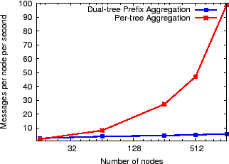
For a 10K-node system, dual tree prefix aggregation reduces the per node
cost of tracking NI from a prohibitive 1000 messages per second
to about 7 messages per second.
messages per time unit.
For a 10K-node system, dual tree prefix aggregation reduces the per node
cost of tracking NI from a prohibitive 1000 messages per second
to about 7 messages per second.
Our NI design separates mechanism from policy and allows applications to use any desired technique to quantify and minimize the impact of disruptions on system reports. For example, in PRISM, monitoring applications use NI to safeguard accuracy by (1) inferring an approximate confidence interval for the number of sensor inputs contributing to a query result, (2) differentiating between correct and erroneous results based on their NI, or (3) correcting distorted results by applying redundancy techniques and then using NI to automatically select the best results. By using NI metrics to filter out inconsistent results and automatically select the best of four redundant aggregation results, we observe a reduction in the worst-case inaccuracy by up to an order of magnitude.
This paper makes five contributions. First, we present Network Imprecision, a new consistency metric that characterizes the impact of network instability on query results. Second, we demonstrate how different applications can leverage NI to detect distorted results and take corrective action.Third, we provide a scalable implementation of NI for DHT overlays via dual-tree prefix aggregation. Fourth, our evaluation demonstrates that NI is vital for enabling scalable aggregation: a system that ignores NI can often silently report arbitrarily incorrect results. Finally, we demonstrate how a distributed monitoring system can both maximize scalability by combining hierarchy, arithmetic filtering, and temporal batching and also safeguard accuracy by incorporating NI.
 |
As discussed in Section 1, large-scale monitoring systems face two key challenges to safeguarding result accuracy. First, node failures, network disruptions, and topology reconfigurations imperil accuracy of monitoring results. Second, common scalability techniques--hierarchical aggregation [5,44,47,53], arithmetic filtering [30,31,36,42,51,56,38], and temporal batching [32,56,36,14]--make the problem worse. In particular, although each technique significantly enhances scalability, each also increases the risk that disruptions will cause the system to report incorrect results.
For concreteness, we describe PRISM's implementation of these techniques although the challenges in safeguarding accuracy are applicable to any monitoring system that operates under node and network failures. We compute a SUM aggregate for all the examples in this section.
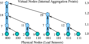
Hierarchical aggregation. Many monitoring systems use hierarchical aggregation [51,47] or DHT-based hierarchical aggregation [5,44,53,39] that defines a tree spanning all nodes in the system. As Figure 1 illustrates, in PRISM, each physical node is a leaf and each subtree represents a logical group of nodes; logical groups can correspond to administrative domains (e.g., department or university) or groups of nodes within a domain (e.g., a /
PRISM leverages
DHTs [44,46,49]
to construct a forest of aggregation trees and maps different
attributes to different
trees
for scalability. DHT systems assign a long (e.g.,
160 bits), random ID to each node and define a routing algorithm to
send a request for ID ![]() to a node
to a node ![]() such that the union of
paths from all nodes forms a tree DHTtree
such that the union of
paths from all nodes forms a tree DHTtree![]() rooted at the node
root
rooted at the node
root![]() . By aggregating an attribute with ID
. By aggregating an attribute with ID ![]() =
hash(attribute) along the aggregation tree corresponding to DHTtree
=
hash(attribute) along the aggregation tree corresponding to DHTtree![]() , different attributes are load balanced across different
trees.
This approach can provide aggregation that
scales to large numbers of nodes and
attributes [53,47,44,5].
, different attributes are load balanced across different
trees.
This approach can provide aggregation that
scales to large numbers of nodes and
attributes [53,47,44,5].
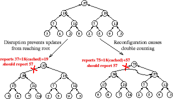 |
Unfortunately, as Figure 2 illustrates, hierarchical aggregation imperils correctness in two ways. First, a failure of a single node or network path can prevent updates from a large collection of leaves from reaching the root, amplifying the effect of the failure [41]. Second, node and network failures can trigger DHT reconfigurations that move a subtree from one attachment point to another, causing the subtree's inputs to be double counted by the aggregation function for some period of time.
Arithmetic Imprecision (AI). Arithmetic imprecision deterministically bounds the difference between the reported aggregate value and the true value. In PRISM, each aggregation function reports a bounded numerical range {
Allowing such arithmetic imprecision enables arithmetic filtering: a subtree need not transmit an update unless the update drives the aggregate value outside the range it last reported to its parent; a parent caches last reported ranges of its children as soft state. Numerous systems have found that allowing small amounts of arithmetic imprecision can greatly reduce overheads [30,31,36,42,51,56].
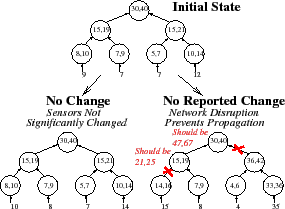 |
Unfortunately, as Figure 3 illustrates, arithmetic filtering raises a challenge for correctness: if a subtree is silent, it is difficult for the system to distinguish between two cases. Either the subtree has sent no updates because the inputs have not significantly changed from the cached values or the inputs have significantly changed but the subtree is unable to transmit its report.
Temporal Imprecision (TI). Temporal imprecision bounds the delay from when an event occurs until it is reported. In PRISM, each attribute has a TI guarantee, and to meet this bound the system must ensure that updates propagate from the leaves to the root in the allotted time.
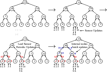 |
As Figure 4 illustrates, TI allows PRISM to use temporal batching: a set of updates at a leaf sensor are condensed into a periodic report or a set of updates that arrive at an internal node over a time interval are combined before being sent further up the tree. Note that arithmetic filtering and temporal batching are complementary: a batched update need only be sent if the combined update drives a subtree's attribute value out of the range previously reported up the tree.
Of course, an attribute's TI guarantee can only be ensured if there is a good path from each leaf to the root. A good path is a path whose processing and propagation times fall within some pre-specified delay budget. Unfortunately, failures, overload, or network congestion can cause a path to no longer be good and prevent the system from meeting its TI guarantees. Furthermore, when a system batches a large group of updates together, a short network or node failure can cause a large error. For example, suppose a system is enforcing TI=60s for an attribute, and suppose that an aggregation node near the root has collected 59 seconds worth of updates from its descendents but then loses its connection to the root for a few seconds. That short disruption can cause the system to violate its TI guarantees for a large number of updates.
This section defines NI and argues that it is the right abstraction for a monitoring system to provide to monitoring applications. The discussions in this section assume that NI is provided by an oracle. Section 4 describes how to compute the NI metrics accurately and efficiently.
The first two properties suggest that traditional data consistency algorithms that enforce guarantees like causal consistency [33] or sequential consistency [34] or linearizability [24] are not appropriate for large-scale monitoring systems. To enforce limits on inconsistency, traditional consistency algorithms must block reads or writes during partitions [19]. However, in large-scale monitoring systems (1) updates cannot be blocked because they reflect external events that are not under the system's control and (2) reads depend on inputs at many nodes, so blocking reads when any sensor is unreachable will result in unacceptable availability.
We therefore cast NI as a monitoring system's introspection on its own stability. Rather than attempt to enforce limits on the inconsistency of data items, a monitoring overlay uses introspection on its current state to produce an NI value that exposes the extent to which system disruptions may affect results.
In its simplest form, NI could be provided as a simple stability flag. If the system is stable (all nodes are up, all network paths are available, and all updates are propagating within the delays specified by the system's temporal imprecision guarantees), then an application knows that it can trust the monitoring system's outputs. Conversely, if the monitoring system detects that any of these conditions is violated, it could simply flag its outputs as suspect, warning applications that some sensors' updates may not be reflected in the current outputs.
Since large systems may seldom be completely stable and
in order to allow different applications sufficient flexibility to
handle system disruptions, instead of an all-or-nothing stability
flag, our implementation of the NI abstraction quantifies the scope of system disruptions.
In particular, we provide three metrics:
![]() ,
,
![]() , and
, and ![]() .
.
Mechanism vs. policy. This formulation of NI explicitly separates the mechanism for network introspection of a monitoring system from application-specific policy for detecting and minimizing the effects of failures, delays, or reconfigurations on query results. Although it is appealing to imagine a system that not only reports how a disruption affects the overlay but also how the disruption affects each monitored attribute, we believe that NI provides the right division of labor between the monitoring system and monitoring applications for three reasons.
First, the impact of omitted or duplicated updates is highly application-dependent, depending on the aggregation function (e.g., some aggregation functions are insensitive to duplicates [12]), the variability of the sensor inputs (e.g., when inputs change slowly, using a cached update for longer than desired may have a modest impact), the nature of the application (e.g., an application that attempts to detect unusual events like network anomalies may reap little value from using statistical techniques for estimating the state of unreachable sensors), and application requirements (e.g., some applications may value availability over correctness and live with best effort answers while others may prefer not to act when the accuracy of information is suspect).
Second, even if it were possible to always estimate the impact of disruptions on applications, hard-wiring the system to do such per-attribute work would impose significant overheads compared to monitoring the status of the overlay.
Third, as we discuss in Section 3.3, there are a broad range of techniques that applications can use to cope with disruptions, and our definition of NI allows each application to select the most appropriate technique.
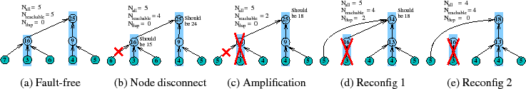 |
Consider the aggregation tree across 5
physical nodes in Figure 5(a).
For simplicity, we compute a SUM aggregate under an
AI filtering budget of zero (i.e., update propagation is suppressed if
the value of an attribute has not changed), and we assume
a TI guarantee of
![]() = 30 seconds (i.e., the system
promises a maximum staleness of 30 seconds). Finally, to avoid
spurious garbage collection/reconstruction of per-attribute state,
the underlying DHT reconfigures its topology if a path
is down for a long timeout (e.g., a few minutes), and internal nodes cache
inputs from their children as soft state for slightly longer
than that amount of time.
= 30 seconds (i.e., the system
promises a maximum staleness of 30 seconds). Finally, to avoid
spurious garbage collection/reconstruction of per-attribute state,
the underlying DHT reconfigures its topology if a path
is down for a long timeout (e.g., a few minutes), and internal nodes cache
inputs from their children as soft state for slightly longer
than that amount of time.
Initially, (a) the system is stable; the root reports the correct
aggregate value of 25 with
![]()
![]()
![]()
![]() 5 and
5 and ![]()
![]() 0 indicating
that all nodes' recent inputs are reflected in the aggregate result with no
duplication.
0 indicating
that all nodes' recent inputs are reflected in the aggregate result with no
duplication.
Then, (b) the input value changes from 7 to 6 at a leaf node, but
before sending that update,
the node gets disconnected from its parent.
Because of soft state caching, the failed
node's old input is still reflected in the SUM aggregate, but
recent changes at that sensor are not;
the root reports 25 but the correct answer is 24.
As (b) shows, NI exposes this inconsistency to the application by
changing
![]() to 4 within
to 4 within
![]() = 30 seconds of the
disruption, indicating that the reported result is based on stale
information from at most one node.
= 30 seconds of the
disruption, indicating that the reported result is based on stale
information from at most one node.
Next, we show how NI exposes the failure amplification effect.
In (c), a single node failure disconnects
the entire subtree rooted at that node.
NI reveals this major disruption by reducing
![]() to 2 since only two leaves retain
a good path to the root. The root still reports 25
but the correct answer (i.e., what an oracle would compute using the
live sensors' values as inputs) is 18.
Since only 2 of 5 nodes
are reachable, this report is suspect.
The application
can either discard it or take corrective actions such as those
discussed in Section 3.3.
to 2 since only two leaves retain
a good path to the root. The root still reports 25
but the correct answer (i.e., what an oracle would compute using the
live sensors' values as inputs) is 18.
Since only 2 of 5 nodes
are reachable, this report is suspect.
The application
can either discard it or take corrective actions such as those
discussed in Section 3.3.
NI also exposes the effects of overlay reconfiguration.
After a timeout, (d) the affected leaves
switch to new parents; NI exposes this change by
increasing
![]() to
4. But since the nodes' old values may still be cached,
to
4. But since the nodes' old values may still be cached,
![]() increases to 2 indicating that two nodes' inputs are
double counted in the root's answer of 34.
increases to 2 indicating that two nodes' inputs are
double counted in the root's answer of 34.
Finally, NI reveals when the system has restabilized.
In (e), the system
again reaches a stable state--the soft state expires,
![]() falls to zero,
falls to zero, ![]() becomes equal to
becomes equal to
![]() of 4,
and the root reports the correct aggregate value of 18.
of 4,
and the root reports the correct aggregate value of 18.
As noted above, NI explicitly separates the problem of characterizing the state of the monitoring system from the problem of assessing how disruptions affect applications. The NI abstraction is nonetheless powerful--it supports a broad range of techniques for coping with network and node disruptions. We first describe four standard techniques we have implemented: (1) flag inconsistent answers, (2) choose the best of several answers, (3) on-demand reaggregation when inconsistency is high, and (4) probing to determine the numerical contribution of duplicate or stale inputs. We then briefly sketch other ways applications can use NI.
Filtering or flagging inconsistent answers. PRISM's first standard technique is to manage the trade-off between consistency and availability [19] by sacrificing availability: applications report an exception rather than returning an answer when the fraction of unreachable or duplicate inputs exceeds a threshold. Alternatively, applications can maximize availability by always returning an answer based on the best available information but flagging that answer's quality as high, medium, or low depending on the number of unreachable or duplicated inputs.
Redundant aggregation. PRISM can aggregate an attribute using
On-demand reaggregation. Given a signal that current results may be affected by significant disruptions, PRISM allows applications to trigger a full on-demand reaggregation to gather current reports (without AI caching or TI buffering) from all available inputs. In particular, if an application receives an answer with unacceptably high fraction of unreachable or duplicated inputs, it issues a probe to force all nodes in the aggregation tree to discard their cached data for the attribute and to recompute the result using the current value at all reachable leaf inputs.
Determine
Since per-attribute ![]() and
and ![]() provide more
information than the NI metrics, which merely characterize the state
of the topology without reference to the aggregation functions or
their values, it is natural to ask: Why not always provide
provide more
information than the NI metrics, which merely characterize the state
of the topology without reference to the aggregation functions or
their values, it is natural to ask: Why not always provide ![]() and
and ![]() and dispense with the NI metrics entirely?
As we will show in Section 4, the NI metrics can be
computed efficiently. Conversely, the attribute-specific
and dispense with the NI metrics entirely?
As we will show in Section 4, the NI metrics can be
computed efficiently. Conversely, the attribute-specific ![]() and
and ![]() metrics must be computed and actively maintained on
a per-attribute basis, making them too expensive for monitoring
a large number of attributes.
Given the range of techniques that can make use of the much
cheaper NI metrics, PRISM provides NI as a general mechanism but allows
applications that require (and are willing to pay for) the more
detailed
metrics must be computed and actively maintained on
a per-attribute basis, making them too expensive for monitoring
a large number of attributes.
Given the range of techniques that can make use of the much
cheaper NI metrics, PRISM provides NI as a general mechanism but allows
applications that require (and are willing to pay for) the more
detailed ![]() and
and ![]() information to do so.
information to do so.
Other techniques. For other monitoring applications, it may be useful to apply other domain-specific or application-specific techniques. Examples include
These examples are illustrative but not comprehensive. Armed with information about the likely quality of a given answer, applications can take a wide range of approaches to protect themselves from disruptions.
The three NI metrics are simple, and implementing them initially seems
straightforward: ![]() ,
,
![]() , and
, and ![]() are each
conceptually aggregates of counts across nodes, which appear to be
easy to compute using PRISM's standard aggregation features. However, this
simple picture is complicated by two requirements on our solution:
are each
conceptually aggregates of counts across nodes, which appear to be
easy to compute using PRISM's standard aggregation features. However, this
simple picture is complicated by two requirements on our solution:
In the rest of this section, we first provide a simple algorithm for
computing ![]() and
and
![]() for a single, static tree. Then, in
Section 4.2, we explain how PRISM computes
for a single, static tree. Then, in
Section 4.2, we explain how PRISM computes ![]() to
account for dynamically changing aggregation topologies.
Later, in Section 4.3 we describe how to scale the
approach to a large number of distinct trees constructed
by PRISM's DHT framework.
to
account for dynamically changing aggregation topologies.
Later, in Section 4.3 we describe how to scale the
approach to a large number of distinct trees constructed
by PRISM's DHT framework.
This section considers calculating ![]() and
and
![]() for a
single, static-topology aggregation tree.
for a
single, static-topology aggregation tree.
![]() is simply a count of all nodes in the system,
which serves as a baseline for evaluating
is simply a count of all nodes in the system,
which serves as a baseline for evaluating
![]() and
and
![]() .
. ![]() is easily computed using PRISM's aggregation abstraction. Each leaf
node inserts 1 to the
is easily computed using PRISM's aggregation abstraction. Each leaf
node inserts 1 to the ![]() aggregate, which has SUM as its
aggregation function.
aggregate, which has SUM as its
aggregation function.
![]() for a subtree is a count of the number of leaves that
have a good path to the root of the subtree, where a good path
is a path whose processing and network propagation times currently fall within
the system's smallest supported TI bound
for a subtree is a count of the number of leaves that
have a good path to the root of the subtree, where a good path
is a path whose processing and network propagation times currently fall within
the system's smallest supported TI bound ![]() . The difference
. The difference
![]()
![]()
![]() thus represents the number of nodes
whose inputs may fail to meet the system's tightest supported staleness
bound; we will discuss what happens for attributes with TI bounds
larger than
thus represents the number of nodes
whose inputs may fail to meet the system's tightest supported staleness
bound; we will discuss what happens for attributes with TI bounds
larger than ![]() momentarily.
momentarily.
Nodes compute
![]() in two steps:
in two steps:
To ensure that
![]() is a lower bound on the number of nodes
whose inputs meet their TI bounds, PRISM processes these probes
using the same data path in the tree as the standard aggregation processing: a
child sends a probe reply only after sending all queued aggregate
updates and the parent processes the reply only after processing all
previous aggregate updates. As a result, if reliable, FIFO network
channels are used, then our algorithm introduces no false negatives:
if probes are processed within their timeouts, then so are all
aggregate updates. Note that our prototype uses
FreePastry [46], which sends updates via unreliable
channels, and our experiments in Section 6 do
detect a small number of false negatives where a responsive node is
counted as reachable even though some recent updates were lost by
the network. We also expect few false positives: since probes and
updates travel the same path, something that delays processing of
probes will likely also affect at least some other attributes.
is a lower bound on the number of nodes
whose inputs meet their TI bounds, PRISM processes these probes
using the same data path in the tree as the standard aggregation processing: a
child sends a probe reply only after sending all queued aggregate
updates and the parent processes the reply only after processing all
previous aggregate updates. As a result, if reliable, FIFO network
channels are used, then our algorithm introduces no false negatives:
if probes are processed within their timeouts, then so are all
aggregate updates. Note that our prototype uses
FreePastry [46], which sends updates via unreliable
channels, and our experiments in Section 6 do
detect a small number of false negatives where a responsive node is
counted as reachable even though some recent updates were lost by
the network. We also expect few false positives: since probes and
updates travel the same path, something that delays processing of
probes will likely also affect at least some other attributes.
Supporting temporal batching. If an attribute's TI bound is relaxed to
To avoid having to calculate a multitude of
![]() values for
different TI bounds, PRISM modifies its temporal batching protocol to
ensure that each attribute's promised TI bound is met for all
nodes counted as reachable. In particular, when a node receives updates from a
child marked unreachable, it knows those updates may be late and may
have missed their propagation window. It therefore marks such
updates as NODELAY. When a node receives a NODELAY update, it
processes the update immediately and propagates the result with the NODELAY
flag so that temporal batching is temporarily suspended for that
attribute. This modification may send extra messages in the
(hopefully) uncommon case of a link performance failure and recovery,
but it ensures that
values for
different TI bounds, PRISM modifies its temporal batching protocol to
ensure that each attribute's promised TI bound is met for all
nodes counted as reachable. In particular, when a node receives updates from a
child marked unreachable, it knows those updates may be late and may
have missed their propagation window. It therefore marks such
updates as NODELAY. When a node receives a NODELAY update, it
processes the update immediately and propagates the result with the NODELAY
flag so that temporal batching is temporarily suspended for that
attribute. This modification may send extra messages in the
(hopefully) uncommon case of a link performance failure and recovery,
but it ensures that
![]() only counts nodes
that are meeting all of their TI contracts.
only counts nodes
that are meeting all of their TI contracts.
Each virtual node in PRISM caches state from its children so that when a new input from one child arrives, it can use local information to compute new values to pass up. This information is soft state--a parent discards it if a child is unreachable for a long time, similar to IGMP [28].
As a result, when a subtree chooses a new parent, that
subtree's inputs may still be stored by a former parent and thus may be
counted multiple times in the aggregate as shown in Figure 5(d).
![]() exposes this inaccuracy by bounding the number
of leaves whose inputs might be included multiple times in the aggregate
query result.
exposes this inaccuracy by bounding the number
of leaves whose inputs might be included multiple times in the aggregate
query result.
The basic aggregation function for ![]() is simple: if a subtree root
spanning
is simple: if a subtree root
spanning ![]() leaves
switches to a new parent, that subtree root inserts the value
leaves
switches to a new parent, that subtree root inserts the value ![]() into the
into the
![]() aggregate, which has SUM as its aggregation function. Later,
when sufficient time has elapsed to ensure that
the node's old parent has removed its soft state, the node
updates its input for the
aggregate, which has SUM as its aggregation function. Later,
when sufficient time has elapsed to ensure that
the node's old parent has removed its soft state, the node
updates its input for the ![]() aggregate to 0.
aggregate to 0.
Our ![]() implementation must deal with two issues.
implementation must deal with two issues.
 |
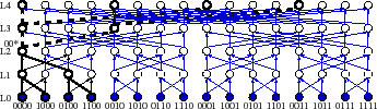
Scaling NI is a challenge. To scale attribute monitoring to a large number of
nodes and attributes, PRISM constructs a forest of trees using an
underlying DHT and then uses different aggregation trees
for different attributes [53,39,44,5].
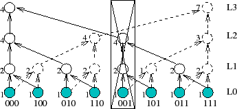
As Figure 6 illustrates, a failure
affects different trees differently. The figure shows two aggregation
trees corresponding to keys 000 and 111 for an 8-node system. In this
system, the failure of the physical node with key 001 removes
only
a leaf node from the tree 111 but disconnects a 2-level subtree
from the tree 000. Therefore,
quantifying the effect of failures requires calculating the NI metrics
for each of the ![]() distinct trees in an
distinct trees in an ![]() -node system.
Making matters worse, as Section 4.1 explained,
maintaining the NI metrics requires frequent active probing along each
edge in each tree.
-node system.
Making matters worse, as Section 4.1 explained,
maintaining the NI metrics requires frequent active probing along each
edge in each tree.
As a result of these factors, the straightforward algorithm for
maintaining NI metrics separately for each tree is not tenable: the DHT forest of
![]() degree-
degree-![]() aggregation trees with
aggregation trees with ![]() physical nodes and each
tree having
physical nodes and each
tree having
![]() edges (
edges (![]() ),
has
),
has
![]() edges that must be monitored; such monitoring would require
edges that must be monitored; such monitoring would require ![]() messages per node per probe interval.
To put this overhead in
perspective, consider a
messages per node per probe interval.
To put this overhead in
perspective, consider a ![]() =1024-node system with
=1024-node system with ![]() =16-ary trees
(i.e., a DHT with 4-bit correction per hop) and a probe interval
=16-ary trees
(i.e., a DHT with 4-bit correction per hop) and a probe interval ![]()
![]()
![]() . The straightforward
algorithm then has each node sending roughly 100 probes per second.
As the system grows, the situation deteriorates rapidly--a 16K-node
system requires each node to send roughly 1600 probes per second.
. The straightforward
algorithm then has each node sending roughly 100 probes per second.
As the system grows, the situation deteriorates rapidly--a 16K-node
system requires each node to send roughly 1600 probes per second.
Our solution, described below, reduces active monitoring work to
![]() probes
per node per second. The 1024-node system in the example would
require each node to send about 5 probes per second; the 16K-node
system would require each node to send about 7 probes per second.
probes
per node per second. The 1024-node system in the example would
require each node to send about 5 probes per second; the 16K-node
system would require each node to send about 7 probes per second.
Dual tree prefix aggregation.To make it practical to maintain the NI values, we take advantage of the underlying structure of our Plaxton-tree-based DHT [44] to reuse common sub-calculations across different aggregation trees using a novel dual tree prefix aggregation abstraction.
 |
As Figure 7
illustrates, this DHT construction forms an approximate butterfly
network. For a
degree-![]() tree, the virtual node at level
tree, the virtual node at level ![]() has an id that matches the
keys that it routes in
has an id that matches the
keys that it routes in
![]() bits. It is the root of exactly one tree,
and its children are approximately
bits. It is the root of exactly one tree,
and its children are approximately ![]() virtual nodes
that match keys in
virtual nodes
that match keys in
![]() bits. It has
bits. It has ![]() parents, each of which
matches different subsets of keys in
parents, each of which
matches different subsets of keys in
![]() bits. But notice that for
each of these parents, this tree aggregates inputs from the same
subtrees.
bits. But notice that for
each of these parents, this tree aggregates inputs from the same
subtrees.
Whereas the standard aggregation abstraction computes a function across a set of subtrees and propagates it to one parent, a dual tree prefix aggregation computes an aggregation function across a set of subtrees and propagates it to all parents. As Figure 7 illustrates, each node in a dual tree prefix aggregation is the root of two trees: an aggregation tree below that computes an aggregation function across nodes in a subtree and a distribution tree above that propagates the result of this computation to a collection of enclosing aggregates that depend on this subtree for input.
For example in Figure 7, consider the level 2
virtual node 00* mapped to node 0000. This node's
![]() count of
4 represents the total number of leaves included in that virtual
node's subtree. This node aggregates this single
count of
4 represents the total number of leaves included in that virtual
node's subtree. This node aggregates this single
![]() count
from its descendants and propagates this value to both of its
level-3 parents, 0000 and 0010. For simplicity, the figure shows a
binary tree; by default PRISM corrects 4 bits per hop, so
each subtree is common to 16 parents.
count
from its descendants and propagates this value to both of its
level-3 parents, 0000 and 0010. For simplicity, the figure shows a
binary tree; by default PRISM corrects 4 bits per hop, so
each subtree is common to 16 parents.
We have developed a prototype of the PRISM monitoring system on top of FreePastry [46]. To guide the system development and to drive the performance evaluation, we have also built three case-study applications using PRISM: (1) a distributed heavy hitter detection service, (2) a distributed monitoring service for Internet-scale systems, and (3) a distribution detection service for monitoring distributed-denial-of-service (DDoS) attacks at the source-side in large-scale systems.
|
Distributed Heavy Hitter detection (DHH). Our first application is identifying heavy hitters in a distributed system--for example, the 10 IPs that account for the most incoming traffic in the last 10 minutes [15,30]. The key challenge for this distributed query is scalability for aggregating per-flow statistics for tens of thousands to millions of concurrent flows in real-time. For example, a subset of the Abilene [1] traces used in our experiments include 260 thousand flows that send about
To scalably compute the global heavy hitters list, we chain two
aggregations where the results from the first feed into
the second. First, PRISM calculates the total
incoming traffic for each destination address from all nodes in the system
using SUM
as the aggregation function and hash(HH-Step1, destIP) as the
key. For example, tuple (H = hash(HH-Step1, 128.82.121.7), 700 KB) at the
root of the aggregation tree ![]() indicates
that a total of 700 KB of data was received for 128.82.121.7 across all vantage points during the last time window. In
the second step, we feed these aggregated total bandwidths for each destination IP into a SELECT-TOP-10 aggregation function with key
hash(HH-Step2, TOP-10) to identify the TOP-10 heavy hitters among all
flows.
indicates
that a total of 700 KB of data was received for 128.82.121.7 across all vantage points during the last time window. In
the second step, we feed these aggregated total bandwidths for each destination IP into a SELECT-TOP-10 aggregation function with key
hash(HH-Step2, TOP-10) to identify the TOP-10 heavy hitters among all
flows.
PRISM is the first monitoring system that we are aware of to combine a scalable DHT-based hierarchy, arithmetic filtering, and temporal batching, and this combination dramatically enhances PRISM's ability to support this type of demanding application. To evaluate this application, we use multiple netflow traces obtained from the Abilene [1] backbone network where each router logged per-flow data every 5 minutes, and we replay this trace by splitting it across 400 nodes mapped to 100 Emulab [52] machines. Each node runs PRISM, and DHH application tracks the top 100 flows in terms of bytes received over a 30 second moving window shifted every 10 seconds.
Figure 8(a) shows the precision-performance results as the AI budget is varied from 0% (i.e., suppress an update if no value changes) to 20% of the maximum flow's global traffic volume and as TI is varied from 10 seconds to 5 minutes. We observe that AI of 10% reduces load by an order of magnitude compared to AI of 0 for a fixed TI of 10 seconds, by (a) culling updates for large numbers of ``mice'' flows whose total bandwidth is less than this value and (b) filtering small changes in the remaining elephant flows. Similarly, TI of 5 minutes reduces load by about 80% compared to TI of 10 seconds. For DHH application, AI filtering is more effective than TI batching for reducing load because of the large fraction of mice flows in the Abilene trace.
PrMon. The second case-study application is PrMon, a distributed monitoring service that is representative of monitoring Internet-scale systems such as PlanetLab [43] and Grid systems that provide platforms for developing, deploying, and hosting global-scale services. For instance, to manage a wide array of user services running on the PlanetLab testbed, system administrators need a global view of the system to identify problematic services (e.g., any slice consuming more than, say, 10GB of memory across all nodes on which it is running.) Similarly, users require system state information to query for lightly-loaded nodes for deploying new experiments or to track and limit the global resource consumption of their running experiments.
To provide such information in a scalable way and in real-time, PRISM computes the per-slice aggregates for each resource attribute (e.g., CPU, MEM, etc.) along different aggregation trees. This aggregate usage of each slice across all PlanetLab nodes for a given resource attribute (e.g., CPU) is then input to a per-resource SELECT-TOP-100 aggregate (e.g., SELECT-TOP-100, CPU) to compute the list of top-100 slices in terms of consumption of the resource.
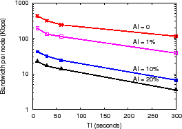
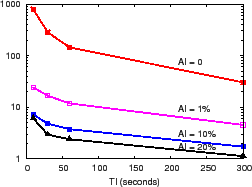
We evaluate PrMon using a CoTop [11] trace from 200 PlanetLab [43] nodes at 1-second intervals for 1 hour. The CoTop data provide the per-slice resource usage (e.g., CPU, MEM, etc.) for all slices running on a node. Using these logs as sensor input, we run PrMon on 200 servers mapped to 50 Emulab machines. Figure 8(b) shows the combined effect of AI and TI in reducing PrMon's load for monitoring global resource usage per slice. We observe AI of 1% reduces load by 30x compared to AI of 0 for fixed TI of 10 seconds. Likewise, compared to TI of 10 seconds and AI of 0, TI of 5 minutes reduces overhead per node by 20x. A key benefit of PRISM's tunable precision is the ability to support new, highly-responsive monitoring applications: for approximately the same bandwidth cost as retrieving node state every 5 minutes (TI = 5 minutes, no AI filtering), PRISM provides highly time-responsive and accurate monitoring with TI of 10 seconds and AI of 1%.
DDoS detection at the source. The final monitoring application is DDoS detection to keep track of which nodes are receiving a large number of traffic (bytes, packets) from PlanetLab. This application is important to prevent PlanetLab from being used maliciously or inadvertently to launch DDoS traffic (which has, indeed, occurred in the past [2]). For input, we collect a trace of traffic statistics--number of packets sent, number of bytes sent, network protocol, source and destination IP addresses, and source and destination ports--every 15 seconds for four hours using Netfilter's connection tracking interface /proc/net/ip_conntrack for all slices from 120 PlanetLab nodes. Each node's traffic statistics are fed into PRISM to compute the aggregate traffic sent to each destination IP across all nodes. Each destination's aggregate value is fed, in turn, to a SELECT-TOP-100 aggregation function to compute a top-100 list of destination IP addresses that receive the highest aggregate traffic (bytes, packets) at two time granularities: (1) a 1 minute sliding window shifted every 15 seconds and (2) a 15 minute sliding window shifted every minute.
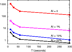
Figure 8(c) shows running the application on 120 PRISM nodes mapped to 30 department machines. The AI budget is varied from 0% to 20% of the maximum flow's global traffic volume (bytes, packets) at both the 1 minute and 15 minutes time windows, and TI is varied from 15 seconds to 5 minutes. We observe that AI of 1% reduces load by 30x compared to AI of 0% by filtering most flows that send little traffic. Overall, AI and TI reduce load by up to 100x and 8x, respectively, for this application.
As illustrated above, our initial experience with PRISM is encouraging: PRISM's load-balanced DHT-based hierarchical aggregation, arithmetic filtering, and temporal batching provide excellent scalability and enable demanding new monitoring applications. However, as discussed in Section 2, this scalability comes at a price: the risk that query results depart significantly from reality in the presence of failures.
This section therefore focuses on a simple question: can NI safeguard accuracy in monitoring systems that use hierarchy, arithmetic filtering, or temporal batching for scalability? We first investigate PRISM's ability to use NI to qualify the consistency guarantees promised by AI and TI, then explore the consistency/availability trade-offs that NI exposes, and finally quantify the overhead in computing the NI metrics. Overall, our evaluation shows that NI enables PRISM to be an effective substrate for accurate scalable monitoring: the NI metrics characterize system state and reduce measurement inaccuracy while incurring low communication overheads.
|
We first illustrate how NI metrics reflect network state in two
controlled experiments in which we run 108 PRISM nodes on Emulab. In
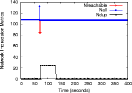
Figure 9(a) we kill a single node 70 seconds
into the run, which disconnects 24 additional nodes from the
aggregation tree being examined. Within
seconds, this failure causes
![]() to fall to 83, indicating
that any result calculated in this interval might only include the
most recent values from 83 nodes. Pastry detects this failure quickly
in this case and reconfigures, causing the disconnected nodes to
rejoin the tree at a new location. These nodes contribute 24 to
to fall to 83, indicating
that any result calculated in this interval might only include the
most recent values from 83 nodes. Pastry detects this failure quickly
in this case and reconfigures, causing the disconnected nodes to
rejoin the tree at a new location. These nodes contribute 24 to
![]() until they are certain that their former parent is no longer
caching their inputs as soft state. The glitch for
until they are certain that their former parent is no longer
caching their inputs as soft state. The glitch for ![]() occurs
because the disconnected children rejoin the system slightly more
quickly than their prior ancestor detects their
departure. Figure 9(b) traces the evolution of
the NI metrics as we kill one of the 108 original nodes every 10 minutes
over a 4 hour run, and similar behaviors are evident; we use higher churn than typical
environments to stress test the system.
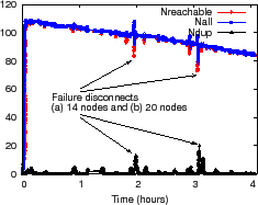
Figure 9(c) shows how NI
reflects network state for a 85-node PrMon experiment on PlanetLab for
an 18-hour run; nodes were randomly picked from 248 Internet2 nodes. For some of the following experiments
we focus on NI's effectiveness during periods of
instability by running experiments on PlanetLab nodes.
Because these nodes show heavy load, unexpected delays, and relatively
frequent reboots (especially prior to deadlines!), we expect these nodes
to exhibit more NI than a typical environment, which
makes them a convenient stress test of our system.
occurs
because the disconnected children rejoin the system slightly more
quickly than their prior ancestor detects their
departure. Figure 9(b) traces the evolution of
the NI metrics as we kill one of the 108 original nodes every 10 minutes
over a 4 hour run, and similar behaviors are evident; we use higher churn than typical
environments to stress test the system.
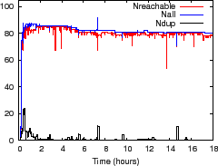
Figure 9(c) shows how NI
reflects network state for a 85-node PrMon experiment on PlanetLab for
an 18-hour run; nodes were randomly picked from 248 Internet2 nodes. For some of the following experiments
we focus on NI's effectiveness during periods of
instability by running experiments on PlanetLab nodes.
Because these nodes show heavy load, unexpected delays, and relatively
frequent reboots (especially prior to deadlines!), we expect these nodes
to exhibit more NI than a typical environment, which
makes them a convenient stress test of our system.
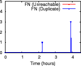
Our implementation of NI is conservative: we are willing to accept
some false positives (when NI reports that inputs are stale or
duplicated when they are not, as discussed in Section 4.1), but we want to minimize false negatives
(when NI fails to warn an application of duplicate or stale inputs).
Figure 10 shows the results for a 96-node Emulab setup under a
network path failure model [13]; we use failure
probability, MTTF, and MTTR of 0.1, 3.2 hours, and 10 minutes.
We contrive an
``append'' aggregation in each of the 96 distinct trees: each node
periodically feeds a (node, timestamp) tuple and internal nodes append
the children inputs together. At each root, we compare the aggregate value
against NI to detect any false positive (FP) or false negative (FN)
reports for (1) ![]() count duplicates and (2)
dips in
count duplicates and (2)
dips in
![]() count nodes whose reported values are
not within TI of their current values.
count nodes whose reported values are
not within TI of their current values.

|
Figure 10 indicates that NI accurately characterizes how churn affects aggregation. Across 300 minutes and 96 trees, we observe fewer than 100 false positive reports, most of them small in magnitude. The high FP near 60 minutes is due to a root failure triggering a large reconfiguration and was validated using logs. We observe zero false negative reports for unreachability and three false negative reports for duplication; the largest error was underreporting the number of duplicate nodes by three. Overall, we observe a FP rate less than 0.3% and a FN rate less than 0.01%.
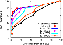
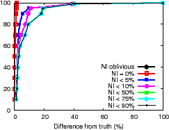
We now examine how applications use NI to
improve their accuracy by compensating for churn. Our basic approach
is to compare results of NI-oblivious aggregation and aggregation with
NI-based compensation with an oracle that has access to
the inputs at all leaves; we simulate the oracle via off-line
processing of input logs. We run a 1 hour trace-based PrMon experiment on 94
PlanetLab nodes or 108 Emulab nodes for a collection of attributes
calculated using a SUM aggregate with AI = 0 and TI = 60 seconds. For
Emulab, we use the synthetic failure model described for Fig 10.
Note
that to keep the discussion simple, we condense NI to a single
parameter: NI =
![]() +
+
![]() for all the subsequent experiments.
for all the subsequent experiments.
|
|
(a) CDF of result accuracy (PlanetLab)
(b) CDF of result accuracy (Emulab)
(c) CDF of observed NI (PlanetLab)
|
The NI-oblivious line of Figure 11(a) and (b) shows for PrMon nodes that ignore NI, the CDF of the difference between query results and the true value of the aggregation computed by an off-line oracle from traces. For PlanetLab, 50% of the reports differ from the truth by more than 30% in this challenging environment. For the more stable Emulab environment, a few results differ from reality by more than 40%. Next, we discuss how applications can achieve better accuracy using techniques discussed in Section 3.3.
Filtering. One technique is to trade availability for accuracy by filtering results during periods of instability. The lines (NI
Filtering answers during periods of high churn exposes a fundamental
consistency versus availability tradeoff [19].
Applications must decide whether it is better to silently give a
potentially inaccurate answer or explicitly indicate when it cannot
provide a good answer. For example, the ![]() line in
Figure 11(c) shows the CDF of the fraction of time for
which NI is at or below a specified value for the PlanetLab run.
For half of the reports, NI
line in
Figure 11(c) shows the CDF of the fraction of time for
which NI is at or below a specified value for the PlanetLab run.
For half of the reports, NI ![]() 30% and for 20% of the reports,
NI
30% and for 20% of the reports,
NI ![]() 80% reflecting high system instability.
Note
that the PlanetLab environment is intended to illustrate
PRISM's behavior during intervals of high churn.
Since accuracy is maximized when answers reflect complete
and current information, systems with fewer disruptions (e.g., Emulab)
are expected to show higher result accuracy compared to PlanetLab and
we observe this behavior for Emulab where
the curves in Figure 11(c)
shift up and to the left
(graph omitted due to space constraints; please see the technical report [31]).
80% reflecting high system instability.
Note
that the PlanetLab environment is intended to illustrate
PRISM's behavior during intervals of high churn.
Since accuracy is maximized when answers reflect complete
and current information, systems with fewer disruptions (e.g., Emulab)
are expected to show higher result accuracy compared to PlanetLab and
we observe this behavior for Emulab where
the curves in Figure 11(c)
shift up and to the left
(graph omitted due to space constraints; please see the technical report [31]).
|
|
(a) PlanetLab redundant aggregation
(b) PlanetLab redundant aggregation + filtering
(c) Emulab redundant aggregation + filtering
|
Redundant aggregation. Redundant aggregation allows applications to trade increased overheads for better availability and accuracy. Rather than aggregating an attribute up a single tree, information can be aggregated up
In Figure 12(a) we explore the effectiveness of a
simple redundant aggregation approach in which PrMon aggregates
each attribute ![]() times and then chooses the result with the lowest
NI. This approach maximizes availability--as long as any of the root
nodes for an attribute are available, PrMon always returns a
result--and it also can achieve high accuracy. Due to space
constraints, we focus on the PlanetLab
run and show the CDF of results with
respect to the deviation from an oracle as we vary
times and then chooses the result with the lowest
NI. This approach maximizes availability--as long as any of the root
nodes for an attribute are available, PrMon always returns a
result--and it also can achieve high accuracy. Due to space
constraints, we focus on the PlanetLab
run and show the CDF of results with
respect to the deviation from an oracle as we vary ![]() from 1 to 4. We
observe that this approach can reduce the deviation to at
most 22% thereby reducing the worst-case inaccuracy by nearly 5x.
from 1 to 4. We
observe that this approach can reduce the deviation to at
most 22% thereby reducing the worst-case inaccuracy by nearly 5x.
Applications can combine the redundant aggregation and filtering techniques to get excellent availability and accuracy. Figure 12(b) and (c) show the results for the PlanetLab and Emulab environments. As Figure 11(c) shows, redundant aggregation increases availability by increasing the fraction of time NI is below the filter threshold, and as Figures 12(b) and (c) show, the combination improves accuracy by up to an order of magnitude over best effort results.
|
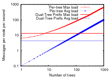
Note that the above experiment constructs all ![]() distinct trees in
the DHT forest of
distinct trees in
the DHT forest of ![]() nodes assuming that the number of attributes
is at least on the order of the number of nodes
nodes assuming that the number of attributes
is at least on the order of the number of nodes ![]() .
However, for systems that aggregate fewer attributes (or if only few attributes care about NI),
it is important to know which of the two techniques
for tracking NI--(1) per-tree aggregation or (2) dual-tree prefix aggregation--is more efficient. Figure 14 shows both the average
and the maximum message cost across all nodes in a 1000-node
experimental setup as above for both per-tree NI aggregation and dual-tree prefix
aggregation as we increase the number of trees along which NI value is
computed. Note that per-tree NI aggregation costs increase as we
increase the number of trees while dual-tree prefix aggregation has a
constant cost. We observe that the break-even point for the average
load is 44 trees while the break-even point for the maximum
load is only 8 trees.
.
However, for systems that aggregate fewer attributes (or if only few attributes care about NI),
it is important to know which of the two techniques
for tracking NI--(1) per-tree aggregation or (2) dual-tree prefix aggregation--is more efficient. Figure 14 shows both the average
and the maximum message cost across all nodes in a 1000-node
experimental setup as above for both per-tree NI aggregation and dual-tree prefix
aggregation as we increase the number of trees along which NI value is
computed. Note that per-tree NI aggregation costs increase as we
increase the number of trees while dual-tree prefix aggregation has a
constant cost. We observe that the break-even point for the average
load is 44 trees while the break-even point for the maximum
load is only 8 trees.
|
The idea of flagging results when the state of a distributed system
is disrupted by node or network failures has been used in tackling
other distributed systems problems. For example, our idea of
NI is analogous to that
of fail-aware services [16]
and failure detectors [9] for fault-tolerant
distributed systems.
Freedman
et al. propose link-attestation groups
[18] that use an application specific
notion of reliability and correctness to map pairs of
nodes which consider each other reliable. Their system, designed for
groups on the scale of tens of nodes, monitors the nodes and system
and exposes such attestation graph to the applications.
Bawa et al. [4] survey previous work on measuring the
validity of query results in faulty networks. Their ``single-site
validity'' semantic is equivalent to PRISM's
![]() metric.
Completeness [20] defined as the percentage of
network hosts whose data contributed to the final query result, is
similar to the ratio of
metric.
Completeness [20] defined as the percentage of
network hosts whose data contributed to the final query result, is
similar to the ratio of
![]() and
and ![]() . Relative
Error [12,57] between the
reported and the ``true'' result at any instant can only be computed
by an oracle with a perfect view of the dynamic network.
. Relative
Error [12,57] between the
reported and the ``true'' result at any instant can only be computed
by an oracle with a perfect view of the dynamic network.
Several aggregation systems have worked to address the failure amplification effect. To mask failures, TAG [36] proposes (1) reusing previously cached values and (2) dividing the aggregate value into fractions equal to the number of parents and then sending each fraction to a distinct parent. This approach reduces the variance but not the expected error of the aggregate value at the root. SAAR uses multiple interior-node-disjoint trees to reduce the impact of node failures [39]. In San Fermin [8], each node creates its own binomial tree by swapping data with other nodes. Seaweed [40] uses a supernode approach in which data on each internal node is replicated. However, both these systems process one-shot queries but not continuous queries on high-volume dynamic data, which is the focus of PRISM. Gossip-based protocols [51,45,7] are highly robust but incur more overhead than trees [53]. NI can also complement gossip protocols, which we leave as future work. Other studies have proposed multi-path routing methods [29,20,12,41,37] for fault-tolerant aggregation.
Recent proposals [37,12,41,4,55] have combined multipath routing with order- and duplicate-insensitive data structures to tolerate faults in sensor network aggregation. The key idea is to use probabilistic counting [17] to approximately count the number of distinct elements in a multi-set. PRISM takes a complementary approach: whereas multipath duplicate-insensitive (MDI) aggregation seeks to reduce the effects of network disruption, PRISM's NI metric seeks to quantify the network disruptions that do occur. In particular, although MDI aggregation can, in principle, reduce network-induced inaccuracy to any desired target if losses are independent and sufficient redundant transmissions are made [41], the systems studied in the literature are still subject to non-zero network-induced inaccuracy due to efforts to balance transmission overhead with loss rates, insufficient redundancy in a topology to meet desired path redundancy, or correlated network losses across multiple links. These issues may be more severe in our environment than in wireless sensor networks targeted by MDI approaches because the dominant loss model may differ (e.g., link congestion and DHT reconfigurations in our environment versus distance-sensitive loss probability for the wireless sensors) and because the transmission cost model differs (for some wireless networks, transmission to multiple destinations can be accomplished with a single broadcast.
The MDI aggregation techniques are also complementary in that PRISM's infrastructure provides NI information that is common across attributes while the MDI approach modifies the computation of individual attributes. As Section 3.3 discussed, NI provides a basis for integrating a broad range of techniques for coping with network error, and MDI aggregation may be a useful technique in cases when (a) an aggregation function can be recast to be order- and duplicate-insensitive and (b) the system is willing to pay the extra network cost to transmit each attribute's updates. To realize this promise, additional work is required to extend MDI approaches for bounding the approximation error while still minimizing network load via AI and TI filtering.
If a man will begin with certainties, he shall end in doubts; but if he will be content to begin with doubts, he shall end in certainties.
-Sir Francis Bacon
We have presented Network Imprecision, a new metric for characterizing network state that quantifies the consistency of query results in a dynamic, large-scale monitoring system. Without NI guarantees, large scale network monitoring systems may provide misleading reports because query result outputs by such systems may be arbitrarily wrong. Incorporating NI in the PRISM monitoring framework qualitatively improves its output by exposing cases when approximation bounds on query results can not be trusted.
This document was generated using the LaTeX2HTML translator Version 2008 (1.71)
Copyright © 1993, 1994, 1995, 1996,
Nikos Drakos,
Computer Based Learning Unit, University of Leeds.
Copyright © 1997, 1998, 1999,
Ross Moore,
Mathematics Department, Macquarie University, Sydney.
The command line arguments were:
latex2html -split 0 -show_section_numbers -local_icons -no_navigation head.tex