Quanto: Tracking Energy in Networked Embedded Systems
Rodrigo Fonseca†⋆, Prabal Dutta†, Philip Levis‡, and Ion Stoica† |
| †Computer Science Division | ⋆Yahoo! Research | ‡Computer Systems Laboratory |
| University of California, Berkeley | Santa Clara, CA | Stanford University |
| Berkeley, CA | Stanford, CA |
Abstract:We present Quanto, a network-wide time and energy profiler for embedded network devices. By combining well-defined interfaces for hardware power states, fast high-resolution energy metering, and causal tracking of programmer-defined activities, Quanto can map how energy and time are spent on nodes and across a network. Implementing Quanto on the TinyOS operating system required modifying under 350 lines of code and adding 1275 new lines. We show that being able to take fine-grained energy consumption measurements as fast as reading a counter allows developers to precisely quantify the effects of low-level system implementation decisions, such as using DMA versus direct bus operations, or the effect of external interference on the power draw of a low duty-cycle radio. Finally, Quanto is lightweight enough that it has a minimal effect on system behavior: each sample takes 100 CPU cycles and 12 bytes of RAM.
Energy is a scarce resource in embedded, battery-operated systems such as sensor networks. This scarcity has motivated research into new system architectures [16], platform designs [17], medium access control protocols [36], networking abstractions [26], transport layers [23], operating system abstractions [21], middleware protocols [11], and data aggregation services [22]. In practice, however, the energy consumption of deployed systems differs greatly from expectations or what lab tests suggest. In one network designed to monitor the microclimate of redwood trees, for example, 15% of the nodes died after one week, while the rest lasted for months [33]. The deployers of the network hypothesize that environmental conditions – poor radio connectivity, leading to time synchronization failure – caused the early demise of these nodes, but a lack of data makes the exact cause unknown.
Understanding how and why an embedded application spends energy requires answering numerous questions. For example, how much energy do individual operations, such as sampling sensors, receiving packets, or using CPU, cost? What is the energy breakdown of a node, in terms of activity, hardware, and time? Network-wide, how much energy do network services such as routing, time synchronization, and localization, consume?
Three factors make these questions difficult to answer. First, nodes need to be able to measure the actual draw of their hardware components.While software models of system energy are reasonably accurate in controlled environments, networks in the wild often experience externalities, such as 100∘ temperature swings [32], electrical shorts due to condensation [31], and 802.11 interference [24]. Second, nodes have limited storage capability, on the order of kilobytes of RAM, and profile collection must be very lightweight, so it is energy efficient and minimizes its effect on system behavior. Finally, there is a semantic gap between common abstractions, such as threads or subsystems, and the actual entities a developer cares about for resource accounting. This gap requires a profiling system to tie together separate operations across multiple energy consumers, such as sampling sensors, sending packets, and CPU operations.
This paper presents Quanto, a time and energy profiler that addresses these challenges through four research contributions. First, we leverage an energy sensor based on a simple switching regulator [9] to enable an OS to take fine-grained measurements of energy usage as cheaply as reading a counter. Second, we show that a post-facto regression can distinguish the energy draw of individual hardware components, thereby only requiring the OS to sample aggregate system consumption. Third, we describe a simple labeling mechanism that causally connects this energy usage to high-level, programmer-defined activities. Finally, we extend these techniques to track network-wide energy usage in terms of node-local actions. We briefly outline these ideas next.
Energy in an embedded system is spent by a set of hardware components operating concurrently, responding to application and external events. As a first step in understanding energy usage, Quanto determines the energy breakdown by hardware component over time. A system has several hardware components, like the CPU, radio, and flash memory, and each one has different functional units, which we call energy sinks. Each energy sink has operating modes with different power draws, which we call power states. At any given time, the aggregate power draw for a system is determined by the set of active power states of its energy sinks.
In many embedded systems, the system software can closely track the hardware components' power states and state transitions. We modify device drivers to track and expose hardware power states to the OS in real-time. The OS combines this information with fine-grained, timely measurements of system-wide energy usage taken using a high-resolution, low-latency energy meter. Every time any hardware component changes its power state, the OS records how much energy was used, and how much time has passed since the immediately preceding power state change. For each interval during which the power states are constant, this generates one equation relating the active power states, the energy used, the time spent, and the unknown power draw of a particular energy sink's power state. Over time, a family of equations are generated and can be solved (i.e. the power draw of individual energy sinks can be estimated) using multivariate linear regression. Section 2 presents the details of this approach.
The next step is to tie together the energy used by different hardware components on behalf of high-level activities such as sensing, routing, or computing, for which we need an abstraction at the appropriate granularity. Earlier work has profiled energy usage at the level of instructions [8], performance events [7], program counter [13], procedures [14], processes [30], and software modules [28]. In this work, we borrow the activity abstraction of a resource principal [2, 19]. An activity is a logical set of operations whose resource usage should be grouped together. In the embedded systems we consider, it is essential that activities span hardware components other than the CPU, and even different nodes.
To account for the resource consumption of activities, Quanto tracks when a hardware component is performing operations on behalf of an activity. Each activity is given a label, and the OS propagates this label to all causally related operations. As an analogy, this tracking is accomplished by conceptually “painting” a hardware component the same “color” as the activity for which it is doing work. To transfer activity labels across nodes, Quanto inserts a field in each packet that includes the initiating activity's label. More specifically, when a packet is passed to the network stack for transmission, the packet's activity field is set to the CPU's then-current activity. This ensures that a transmitted packet is labeled the same as the activity which initiated its submission. Upon reception, Quanto reads the packet's hidden field and sets the CPU activity to the activity noted in the packet. In Section 3 we give a more precise definition of activities, and detail how Quanto implements activity tracking across both the hardware components of a single node and across the nodes in a network.
The final step is to merge this information. Quanto records events for both power state and activity changes for each hardware resource. In our current prototype, we use these logs to perform this step post-facto. From the power states log and the regression, we know the active power state and the power draw for each hardware component; from the activities log, we know on behalf of which activity the component was doing work. Combining these two pieces of information provides a thorough breakdown of energy consumption over time.
To evaluate the functionality and performance of Quanto, we implemented the framework in TinyOS, a popular sensornet operating system. Implementing our approach required small changes to six OS abstractions – timers, tasks, arbiters, network stack, interrupt handlers, and device drivers. We changed 22 files and 171 lines of code for core OS primitives, and 16 files and 148 lines of code for representative device drivers, to support activity tracing and exposing of power states.
In this section, we present how Quanto answers the question where have all the joules gone? This requires distinguishing the individual energy consumption of hardware components or peripherals that are operating concurrently when only their aggregate energy usage is observable. We ground our discussion on the specific hardware and software platform in our prototype, although we believe the techniques to be applicable to other platforms as well. We briefly sketch our approach in the next subsection and then use the remainder of this section to describe Quanto's energy tracking framework in detail.
In many embedded systems, the OS can track the power states and state transitions of the platform's various energy sinks. This power state information can be combined with snapshots of the aggregate energy consumption to infer the consumption of individual sinks.
We call each functional unit in a system an energy sink, and their different operating modes power states. Quanto modifies the device drivers to intercept all events which change the power state of an energy sink. The OS itself keeps track of both the energy usage, Δ E, and elapsed time, Δ t, between any two such events. Since the OS tracks the active sinks and their power states, it is able to generate one linear equation of the following form for each interval
| Δ E = Δ t |
| αi pi (1) |
where the average power over the interval, P, is Δ E/Δ t. The variable αi is a binary variable indicating whether the i-th power state was active during the interval, and pi is the (unknown) power draw of the i-th state. The limit n represents the total number of power states over all energy sinks in the system. In one time interval, this equation is not solvable (unless only one power state is active), but over time, an application generates a system of equations as different energy sinks transition through different power states. When the system of equations is sufficiently constrained, a simple linear regression yields the individual power draws.
Because it samples the accumulated energy consumption at every hardware power state change, Quanto requires high-resolution, low-latency, and low-overhead energy measurements. These readings must closely reflect the energy consumed during the preceding interval. To accomplish this, our implementation uses the iCount energy meter [9]. The iCount implementation on this platform exhibits a maximum error of ±15% over five orders of magnitude in current draw, an energy resolution of approximately 1 µJ, a read latency of 24 µs (24 instruction cycles), and a power overhead that ranges from 1% when the node is in standby to 0.01% when the node is active, for a typical workload.
We used the HydroWatch platform which incorporates iCount into a custom sensornet node [10]. This platform uses the Texas Instruments 16-bit MSP430F1611 microcontroller with 48 KB of internal flash memory and 10 KB of RAM, an 802.15.4-compliant CC2420 radio, and an Atmel 16-Mbit AT45DB161D NOR flash memory. The platform also includes three LEDs.
The Hydrowatch platform's energy sinks, and their nominal current draws, are shown in Table 1. The microcontroller includes several different functional units. The microcontroller's eight energy sinks have sixteen power states but since many of the energy sinks can operate independently, the microcontroller can exhibit hundreds of distinct draw profiles. The five energy sinks in the radio have fourteen power states. Some of these states are mutually exclusive. For example, the radio cannot use both receive and transmit at the same time. Similarly, the flash memory can operate in several distinct power states. Collectively, the energy sinks represented by the microcontroller, radio, flash memory, and LEDs can operate independently, so, in principle, the system may exhibit hundreds or thousands of distinct power profiles.
Energy Sink Power State Current Microcontroller CPU ACTIVE 500 µA LPM0 75 µA LPM1† 75 µA LPM2 17 µA LPM3 2.6 µA LPM4 0.2 µA Voltage Reference ON 500 µA ADC CONVERTING 800 µA DAC CONVERTING-2 50 µA CONVERTING-5 200 µA CONVERTING-7 700 µA Internal Flash PROGRAM 3 mA ERASE 3 mA Temperature Sensor SAMPLE 60 µA Analog Comparator COMPARE 45 µA Supply Supervisor ON 15 µA Radio Regulator OFF 1 µA ON 22 µA POWER_DOWN 20 µA Batter Monitor ENABLED 30 µA Control Path IDLE 426 µA Rx Data Path RX (LISTEN) 19.7 mA Tx Data Path TX (+0 dBm) 17.4 mA TX (-1 dBm) 16.5 mA TX (-3 dBm) 15.2 mA TX (-5 dBm) 13.9 mA TX (-7 dBm) 12.5 mA TX (-10 dBm) 11.2 mA TX (-15 dBm) 9.9 mA TX (-25 dBm) 8.5 mA Flash POWER_DOWN 9 µA STANDBY 25 µA READ 7 mA WRITE 12 mA ERASE 12 mA LED0 (Red) ON 4.3 mA LED1 (Green) ON 3.7 mA LED2 (Blue) ON 1.7 mA
Table 1: The platform energy sinks, their power states, and the nominal current draws in those states at a supply voltage of 3 V and clock speed of 1 MHz, compiled from the datasheets. †Assumed.
Tracking power states involves a collaborative effort between device drivers and the OS: we modify the device driver that abstracts a hardware resource to expose the device power states through a simple interface, while the OS tracks and logs the power states across the system.
Quanto defines the PowerState interface, shown in Figure 1, and provides a generic component that implements it. A device driver merely declares that it uses this interface and signals hardware power state changes through its simple calls. This approach eliminates state tracking in many device drivers and simplifies the instrumentation of more complex device drivers. Multiple calls to the PowerState interface signaling the same state are idempotent: such calls do not result in multiple notifications to the OS.
Figure 2 illustrates the changes to the LED device driver to expose power states. This requires intercepting calls to turn the LED on and off and notifying the OS of these events. For a simple device like the LED which only has two states and whose power states are under complete control of the processor, exposing the power state is a simple and relatively low-overhead matter.
interface PowerState {
  // Sets the powerstate to value.
  async command void set(powerstate_t value);

  // Sets the bits represented by mask to value.
  async command void setBits(powerstate_t mask,
    uint8_t offset, powerstate_t value);
}
Figure 1: Device drivers must be modified to expose device power states using the PowerState interface.
async command void Leds.led0On() {
  call Led0PowerState.set(1);
  // Setting pin to low turns Led on
  call Led0.clr();
}

async command void Leds.led0Off() {
  call Led0PowerState.set(0);
  // Setting pin to high turns Led off
  call Led0.set();
}
Figure 2: Implementing power state tracking is simple for many devices, like LEDs, and requires signaling power state changes using the PowerState interface.
interface PowerStateTrack {
  // Called if an energy sink power state changes
  async event void changed(powerstate_t value);
}
Figure 3: The PowerStateTrack interface is used by the OS and applications to receive power state change events in real-time.
More involved changes to the device driver are needed if a device's power state can change outside of direct CPU control. Flash memory accesses, for example, go through a handshaking process during which the power states and transitions are visible to the processor but not directly controlled by it. Prior to a write request, a flash chip may be in an idle or sleep state. When the processor asserts the flash chip enable line, the flash transitions to a ready state and asserts the ready line. Upon detecting this condition, the processor can issue a write command over a serial bus, framed by a write line assertion. The flash may then signal that it is busy writing the requested data by asserting the busy signal. When finished with the write, the flash asserts the ready signal. In this example, the device driver should monitor hardware handshake lines or use timeouts to shadow and expose the hardware power state.
The glue between the device drivers and OS is a component that exposes the PowerState interface to device drivers and provides the PowerStateTrack interface, shown in Figure 3, to the OS and application. This component tracks the power states change events and only notifies the OS and registered application listeners when an actual state change occurs. Each time a power state changes, Quanto logs the current value of the energy meter, the time, and the vector of power states.
The purpose of estimating the energy breakdown is to attribute to each energy sink its share of the energy consumption. Quanto uses weighted multivariate least squares to estimate the power draw of each energy sink. The input to this offline regression process is a log that records, for each interval during which the power states are same, the aggregate energy consumed during that interval (Δ E), the length of the interval (Δ t), and the power states of all devices during the interval (α1,…,αn).
We estimate the power draw of the i-th energy sink as follows. First we group all intervals from the log that have the same power state j (a particular setting of α1,…,αn), adding the time tj and energy Ej spent at that power state. For each power state j, possibly ranging from 1 to 2n, we determine the average aggregate power yj:
| yj = Ej/ tj, |
and collect them in a column vector Y over all j:
| Y= |
| . |
Due to quantization effects in both our time and energy measurements, the confidence in yj increases with both Ej and tj. Correspondingly, we use a weight, wj=√Ejtj for each estimate in the regression, and group them in a diagonal weight matrix W. We use the square root because, for a constant power level, Ej and tj are linearly dependent.
We first collect the observed power states αj,i in a matrix X:
| X= |
|
Then, the unknown power draws are estimated:
| Π = (XTWX)−1XTWY, |
and finally, the residual errors are given by:
| є = Y−XΠ |
Tracking power states and energy consumption of energy sinks over time shows where and when the energy is going, but leaves a semantic gap to the programmer of why the energy is being spent.
The key here is to attribute energy usage to entities – or resource principals – that are meaningful to the programmer. In traditional operating systems, processes or threads combine the roles of protection domain, schedulable unit, and resource principal, but there are many situations in which it is desirable that these notions be independent. This idea was previously explored in the context of high-performance network servers [2] but it is also especially true in networked embedded systems.
We borrow from earlier work the concept of an activity as our resource principal. In the Rialto system in particular [19], an activity was defined as the “the abstraction to which resources are allocated and to which resource usage is charged.” In other words, an activity is a set of operations whose resource consumption should be grouped together. In the environments we consider, where most of the resource consumption does not happen at the CPU, and sometimes not even on the same node that initiated an activity, it is fundamental to support activities that span different hardware components and multiple nodes.
We close the gap of why energy is spent by assigning the energy consumption to activities that are defined by the programmer at a high level. To do this we follow all operations related to an activity across hardware components on a single node and across the network.
To account for the resource consumption of activities, we track when a hardware component, or device, is performing operations on behalf of an activity. A useful analogy is to think of an activity as a color, and devices as being painted with the activity's color when working on its behalf. By properly recording devices' successive colors over time and their respective resource consumptions, we can assign to each activity its share of the energy usage.
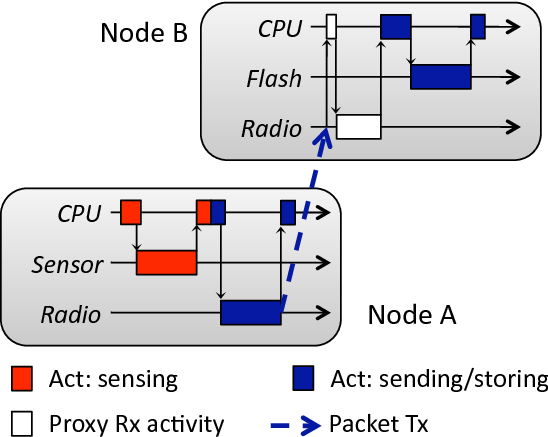
Figure 4 shows an example of how activities can span multiple devices and nodes. In the figure, the programmer marks the start of an activity by assigning to the CPU the sensing activity (“painting the CPU red”). We represent activities by activity labels, which Quanto carries automatically to causally related operations. For example, when a CPU that is “painted red” invokes an operation on the sensor, the CPU paints the sensor red as well. The programmer may decide to change the CPU activity if it starts work on behalf of a new logical activity, such as when transitioning from sensing to sending (red to blue in the figure). Again the system will propagate the new activity to other devices automatically.
This propagation includes carrying activity labels on network messages, such that operations on node B can be assigned to the activity started on node A. This example also highlights an important aspect of the propagation, namely proxy activities. When the CPU on node B receives an interrupt indicating that the radio is starting to receive a packet, the activity to which the receiving belongs is not known. This is generally true in the case of interrupts and external events. Proxy activities are a solution to this problem. The resources used by a proxy activity are accounted for separately, and then assigned to the real activity as soon as the system can determine what this activity is. In this example the CPU can determine that it should be colored blue as soon as it decodes the activity label in the radio packet. It terminates the proxy activity by binding it to the blue activity.
The programmer can define the granularity of activities in a flexible way, guided by how she wants to divide the resource consumption of the system. Some operations do not clearly belong to specific activities, such as data structure maintenance or garbage collection. One option is to give these operations their own activities, representing this fact explicitly.
The mechanisms for tracking activities are divided into three parts, which we describe in more detail next, in the context of TinyOS: (i) an API that allows the programmer to create meaningful activity labels, (ii) a set of mechanisms to propagate these labels along with the operations that comprise the activity, (iii) and a mechanism to account for the resources used by the activities.
We represent activity labels with pairs of the form <origin node:id>, where id is a statically defined integer, and origin node indicates the node where the activity starts.
We provide an API that allows the assignment of activity labels to devices over time. This API is shown in Figures 5 and 6, respectively, for devices that can only be performing operations on behalf of one, or possibly multiple activities simultaneously. Most devices, including CPUs, are SingleActivityDevices.
interface SingleActivityDevice {
  // Returns the current activity
  async command act_t get();

  // Sets the current activity
  async command void set(act_t newActivity);

  // Sets the current activity and indicates
  // that the previous activity's resource
  // usage should be charged to the new one
  async command void bind(act_t newActivity);
}
Figure 5: The SingleActivityDevice interface. This interface represents hardware components that can only be part of one activity at a time, such as the CPU or the transmit part of the radio.
interface MultiActivityDevice {
  // Adds an activity to the set of current
  // activities for this device
  async command error_t add(act_t activity);

  // Removes an activity from the set of current
  // activities for this device
  async command error_t remove(act_t activity);
}
Figure 6: The MultiActivityDevice interface. This interface represents hardware components that can be working simultaneously on behalf of multiple activities. Examples include hardware timers and the receiver circuitry in the radio (when listening).
There are two classes of users for the API, application programmers and system programmers. Application programmers simply have to define the start of high-level activities, and assign labels to the CPU immediately before their start. System programmers, in turn, use the API to propagate activities in the lower levels of the system such as device drivers. We instrumented core parts of the OS, such as interrupt routines, the scheduler, arbiters [21], the network stack, radio, and the timer system. Figure 7 shows an excerpt of a sense-and-send application similar to the one described in [21], in which the application programmer “paints” the CPU using the CPUActivity.set method (an instance of the SingleActivityDevice interface) before the start of each logical activity. The OS takes care of correctly propagating the labels with the following execution.
task void sensorTask() {
  call CPUActivity.set(ACT_HUM);
  call Humidity.read();
  call CPUActivity.set(ACT_TEMP);
  call Temperature.read();
}

void sendIfDone() {
  if (sensingDone) {
    call CPUActivity.set(ACT_PKT);
    post sendTask();
    sensingDone = 0;
  }
}
Figure 7: Excerpt from a sense-and-send application, showing how an application programmer “paints” the CPU to start tracking activities.
Once we have application level activities set by the application programmer, the OS has to carry activity labels to all operations related to each activity. This involves 4 major components: (i) transfer activity labels across devices, (ii) transfer activity labels across nodes, (iii) bind proxy activities to real activities when interrupts occur, and (iv) follow logical threads of computation across several control flow deferral and multiplexing mechanisms.
To transfer activity labels across devices our instrumentation of TinyOS uses the Single- and MultiActivityDevice APIs. Each hardware component is represented by one instantiation of such interfaces, and keeps the activity state for that component globally accessible to code. The CPU is represented by a SingleActivityDevice, and is responsible for transferring activity labels to and from other devices. An example of this transfer is shown in Figure 8, where the code “paints” the radio device with the current CPU activity. Device drivers must be instrumented to correctly transfer activities between the CPU and the devices they manage. In our prototype implementation we instrumented several devices, including the CC2420 radio and the SHT11 sensor chip. Also, we instrumented the Arbiter abstraction [21], which controls access to a number of shared hardware components, to automatically transfer activity labels to and from the managed device.
To transfer activity labels across nodes, we added a hidden field to the TinyOS Active Message (AM) implementation (the default communication abstraction). When a packet is submitted to the OS for transmission, the packet's activity field is set to the CPU's current activity. This ensures the packet is colored the same as the activity which initiated its submission. We currently encode the labels as 16-bit integers representing both the node id and the activity id, which is sufficient for networks of up to 256 nodes with 256 distinct activity ids. Upon decoding a packet, the AM layer on the receiving node sets the CPU activity to the activity in the packet, and binds resources used between the interrupt for the packet reception and the decoding to the same activity.
More generally, this type of resource binding is done when we have interrupts. Our prototype implementation uses the Texas Instruments MSP430F1611 microcontroller. Since TinyOS does not have reentrant interrupts on this platform, we statically assign to each interrupt handling routine a fixed proxy activity. An interrupt routine temporarily sets the CPU activity to its own proxy activity, and the nature of interrupt processing is such that very quickly, in most cases, we can determine to which real activity the proxy activity should be bound. One example is the decoding of the radio packets at the Active Message layer. Another example is an interrupt caused by a device signaling the completion of a task. In this case, the device driver will have stored locally both the state required to process the interrupt and the activity to which this processing should be assigned.
Lastly, the propagation of activity labels should follow the control flow of the logical threads of execution across deferral and multiplexing mechanisms. The most important and general of these mechanisms in TinyOS are tasks and timers.
TinyOS has a single stack, and uses an event-based execution model to multiplex several parallel activities among its components. The schedulable unit is a task. Tasks run to completion and do not preempt other tasks, but can be preempted by asynchronous events triggered by interrupts. To achieve high degrees of concurrency, tasks are generally short lived, and break larger computations in units that schedule each other by posting new tasks. We instrumented the TinyOS scheduler to save the current CPU activity when a task is posted, and restore it just before giving control to the task when it executes, thereby maintaining the activities bound to tasks in face of arbitrary multiplexing. Timers are also an important control flow deferral mechanism, and we instrumented the virtual timer subsystem to automatically save and restore the CPU activity of scheduled timers.
There are other less general structures that effectively defer processing of an activity, such as forwarding queues in protocols, and we have to instrument these to also store and restore the CPU activity associated with the queue entry. As we show in Section 4, changes to support propagation in a number of core OS services were small and localized.
void loadTXFIFO() {
  ...
  //prepare packet
  ...
  call RadioActivity.set(call CPUActivity.get());
  call TXFIFO.write((uint8_t*)header,
                    header->length - 1);
}
Figure 8: Excerpt from the CC2420 transmit code that loads the TXFIFO with the packet data. The instrumentation sets the RadioActivity to the current value of the CPUActivity.
The final element of activity tracking is recording the usage of resources for accounting and charging purposes. Similarly to how we track power states, we implement the observer pattern through the SingleActivityTrack and MultiActivityTrack interfaces (Figure 9). These are provided by a module that listens to the activity changes of devices and is currently connected to a logger. In our prototype we log these events to RAM and do the accounting offline. For single-activity devices, this is straightforward, as time is partitioned among activities. For multi-activity devices, the the log records the set of activities for a device over time, and how to divide the resource consumption among the activities for each period is a policy decision. We currently divide resources equally, but other policies are certainly possible.
interface SingleActivityTrack {
  async event void changed(act_t newActivity);
  async event void bound(act_t newActivity);
}
interface MultiActivityTrack {
  async event void added(act_t activity);
  async event void removed(act_t activity);
}
Figure 9: Single- and MultiActivityTrack interfaces provided by device abstractions. Different accounting modules can listen to these events.
In this section we first look at two simple applications, Blink and Bounce, that illustrate how Quanto combines activity tracking, power-state tracking, and energy metering into a complete energy map of the application. We use the first, Blink, to calibrate Quanto against ground truth provided by an oscilloscope, and as an example of a multi-activity, single-node application. We use the second, Bounce, as an example with activities that span different nodes. We then look at three case studies in which Quanto exposes real-world effects and costs of application design decisions, and lastly we quantify some of the costs involved in using Quanto itself. In these experiments processed Quanto data with a set of tools we wrote to parse and visualize the logs. We used GNU Octave to perform the regressions.
We set up a simple experiment to calibrate Quanto against the ground truth provided by a digital oscilloscope. The goal is to establish that Quanto can indeed measure the aggregate energy used by the mote, and that the regression does separate this energy use by hardware components.
We use Blink, the hello world application in TinyOS. Blink is very simple; it starts three independent timers with intervals of 1, 2, and 4s. When these timers fire, the red, green, and blue LEDs are toggled, such that in 8 seconds Blink goes through 8 steady states, with all combinations of the three LEDs on and off. The CPU is in its sleep state during these steady states, and only goes active to perform the transitions.
Using the Hydrowatch board (cf. Section 2.2), we connected a Tektronix MSO4104 oscilloscope to measure the voltage across a 10 resistor inserted between iCount circuit and the mote power input. We measured the voltage provided by the regulator for the mote to be 3.0V.
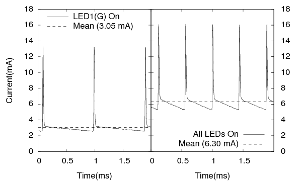
We confirmed the result from [9] that the switching frequency of iCount varies linearly with the current. Figure 10 shows the current for two sample states of Blink. This curve has a wealth of information: from it we can derive both the switching frequency of the regulator, which is what Quanto measures directly, and the actual average current, Iavg. We verified over the 8 power states that Iavg, in mA, and the switching frequency fiC, in kHz, have a linear dependency given by Iavg = 2.77fiC−0.05, with an R2 value of 0.99995. We can infer from this that each iCount pulse corresponds, in this hardware, at 3 V, to 8.33 uJ. We also verified that Iavg was stable during each interval.
X Y L0 L1 L2 C I(mA) 0 0 0 1 0.74 1 0 0 1 3.32 0 1 0 1 3.05 1 1 0 1 5.53 0 0 1 1 1.62 1 0 1 1 4.15 0 1 1 1 3.88 1 1 1 1 6.30
Π I(mA) LED0 2.50 LED1 2.23 LED2 0.83 Const. 0.79
XΠ I(mA) 0.79 3.29 3.02 5.53 1.62 4.12 3.85 6.36
Table 2: Oscilloscope measurements of the current for the steady states of Blink, and the results of the regression with the current draw per hardware component. The relative error (||Y−XΠ||/||Y||) is 0.83%.
Lastly we tested the regression methodology from Section 2.5, using the average current measured by the oscilloscope in each state of Blink and the external state of the LEDs as the inputs. We also added a constant term to account for any residual current not captured by the LED state. Table 2 shows the results, and the small relative error indicates that for this case the linearity assumptions hold reasonably well, and that the regression is able to produce a good breakdown of the power draws per hardware device.
(a) Time break down.
Hardware Components - Time(s) Activities LED0 LED1 LED2 CPU 1:Red 24.01 0 0 0.0176 1:Green 0 24.00 0 0.0091 1:Blue 0 0 24.00 0.0045 1:Vtimer 0 0 0 0.0450 1:int_Timer 0 0 0 0.0092 1:Idle 23.99 24.00 24.00 47.9169 Total 48.00 48.00 48.00 48.0024 (b) Result of the regression.
Hardware Components - Π LED0 LED1 LED2 CPU Const. Iavg(mA) 2 . 51 2.24 0.83 1.43 0.83 Pavg(mW) 7 . 53 6.71 2.49 4.29 2.48 (c) Total Energy per Hardware Component.
∑EHW(mJ) LED0 180 . 71 LED1 161 . 06 LED2 59 . 84 CPU 0 . 37 Const. 119 . 26 Total 521 . 23 (d) Total Energy per Activity.
Activities ∑Eact(mJ) 1:Red 180 . 78 1:Green 161 . 10 1:Blue 59 . 86 1:Vtimer 0 . 19 1:int_Timer 0 . 04 1:Idle 0 . 00 Const. 119 . 26 Total 521 . 23
Table 3: Where the joules have gone in Blink. The tables show how activities spend time on hardware components (a), the regression results (b), and a break down of the energy usage by activity (c) and hardware component (d).
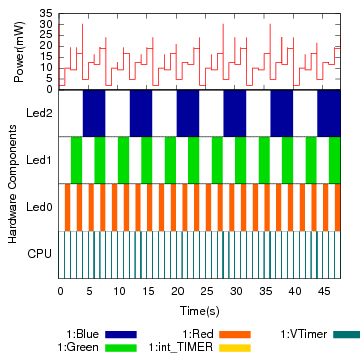
(a) Power draw measured by Quanto and the activities over time for each hardware component.
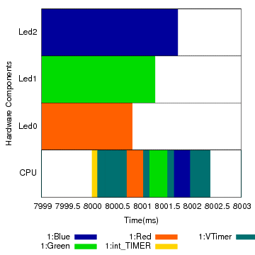
(b) Detail of a transition from all on to all off, showing the activities for each hardware component.
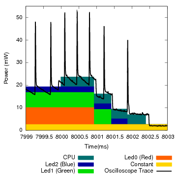
(c)Stacked power draw for the hardware components, with values from the regression, overlaid with the oscilloscope-measured power.
Figure 11: Activity and power profiles for a 48-second run of the Blink application on the Hydrowatch platform.
We instrumented Blink with Quanto to verify the results from the calibration and to demonstrate a simple case of tracking multiple activities on a single node. We divided the application into 3 main activities: Red, Green, and Blue, which perform the operations related to toggling each LED. Each LED, when on, gets labeled with the respective activity by the CPU, such that its energy consumption can be charged to the correct activity. We also created an activity to represent the managing of the timers by the CPU (VTimer). We recorded the power states of each LED (simply on and off), and consider the CPU to only have two states as well: active, and idle.
Figures 11(a) and (b) show details of a 48-second run of Blink. In these plots, the X axis represents time, and each color represents one activity. The lower part of (a) shows how each hardware component divided its time among the activities. The topmost portion of the graph shows the aggregate power draw measured by iCount. There are eight distinct stable draws, corresponding to the eight states of the LEDs.
Part (b) zooms in on a particular state transition spanning 4 ms, around 8 s into the trace, when all three LEDs simultaneously go from their on to off state, and cease spending energy on behalf of their respective activities. At this time scale it is interesting to observe the CPU activities. For clarity, we did not aggregate the proxy activities from the interrupts into the activities they are bound to. At 8.000 s the timer interrupt fires, and the CPU gets labeled with the int_TIMERB0 and VTimer activities. VTimer, after examining the scheduled timers, yields to the Red, Green, and Blue activities in succession. Each activity turns off its respective LED, clears its activities, and sets its power state to off. VTimer performs some bookkeeping and then the CPU sleeps.
Table 3(a) shows, for the same run, the total time when each hardware component spent energy on behalf of each activity. The CPU is active for only 0.178% of the time. Also, although the LEDs stay on for the same amount of time, they change state a different number of times, and the CPU time dedicated to each corresponding activity reflects that overhead.
We ran the regression as described in Section 2.5 to identify the power draw of each hardware component. Table 3(b) shows the result in current and power. This information, combined with the time breakdown, allows us to compute the energy breakdown by hardware component (c), and by activity (d). The correlation between the corresponding components of Table 3(b) and the current breakdown in Table 2 is 0.99988. Note that we don't have the CPU component in the oscilloscope measurements because it was hard to identify in the oscilloscope trace exactly when the CPU was active, something that is easy with Quanto.
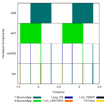
(a) A 2-second window on a run of Bounce at a node with id 1.
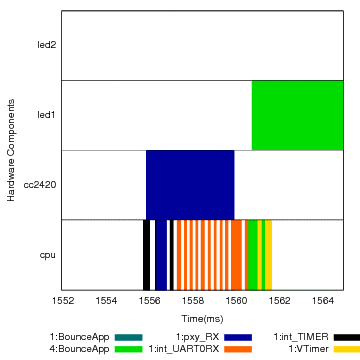
(b) Detail of a packet reception with an activity label from node 4.
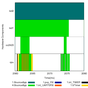
(c) Detail of a packet transmission on node 1 as part of the activity started at node 4.
Figure 12: Activity tracking on Bounce. Each packet carries the activity current at the time it was generated, and the receiving node executes some operations as part of that remote activity.
From the power draw of the individual hardware components we can reconstruct the power draw of each power state and verify the quality of the regression. The relative error between the total energy measured by Quanto and the energy derived from the reconstructed power state traces was 0.004% for this run of Blink.
Figure 11(c) shows a stacked breakdown of the measured energy envelope, reconstructed from the power state time series and the results of the regression. The shades in this graph represent the different hardware components, and at each interval the stack shows which components are active, and in what proportion they contribute to the overall energy consumption. The graph also shows an overlaid power curve measured with the oscilloscope for the same run. The graph shows a very good match between the two sources, both in the time and energy dimensions. We can notice small time delays between the two curves, on the order of 100 µs, due to the time Quanto takes to record a measurement.
The second example we look at illustrates how Quanto keeps track of activities across nodes. Bounce is a simple application in which two nodes keep exchanging two packets, each one originating from one of the nodes. In this example we had nodes with ids 1 and 4 participate. All of the work done by node 1 to receive, process, and send node 4's original packet is attributed to the '4:BounceApp' activity. Although this is a trivial example, the same idea applies to other scenarios, like protocol beacon messages and multihop routing of packets.
Figure 12 shows a 2-second trace from node 1 of a run of Bounce. The log at the other node is symmetrical. On part (a) we see the entire window, and the activities by the CPU, the radio, and two LEDs that are on when the node has “possession” of each packet. In this figure, node 1 receives a packet which carries the 4:BounceApp activity, and turns LED1 on because of that. The energy spent by this LED will be attributed to node 4's original activity. The node then receives another packet, which carries its own 1:BounceApp activity. LED2's energy spending will be assigned to node 1's activity, as well as the subsequent transmission of this same packet.
Figures 12(b) and (c) show in detail a packet reception and transmission, and how activity tracking takes place in these two operations. Again, we keep the interrupt proxy activities separated, although when accounting for resource consumption we should assign the consumption of a proxy activity to the activity to which it binds. The receive operation starts with a timer interrupt for the start of frame delimiter, followed by a long transfer from the radio FIFO buffer to the processor, via the SPI bus. This transfer uses an interrupt for every 2 bytes. When finished, the packet is decoded by the radio stack, and the activity in the packet can be read and assigned to the CPU. The CPU then “paints” the LED with this activity and schedules a timer to send the packet.
Transmission in Bounce is triggered by a timer interrupt that was scheduled upon receive. The timer carries and restores the activity, and “paints” the radio. There are two main phases for transmission. First, the data is transferred to the radio via the SPI bus, and then, after a backoff interval, the actual transmission happens. When the transmission is done, the CPU then turns the LED off and sets its activity to idle.
Quanto allows a developer to precisely understand and quantify the effects of design decisions, and we discuss three case studies from the TinyOS codebase.
The first one is an investigation of the effect of interference from an 802.11 b/g network on the operation of low-power listening [25]. Low-power listening (LPL) is a family of duty-cycle regimes for the radio in which the receiver stays mostly off, and periodically wakes up to detect whether there is activity on the channel. If there is, it stays on to receive packets, otherwise it goes back to sleep. In the simplest version, a sender must transmit a packet for an interval as long as the receiver's sleep interval. A higher level of energy in the channel, due to interference from other sources, can cause the receiver to falsely detect activity, and stay on unnecessarily. Since 802.11 b/g and 802.15.4 radios share the 2.4 GHz band, and the former generally has much higher power than the latter, this scenario can be quite common. We used Quanto to measure the impact of such interference. We set an 802.11 b access point to operate on channel 6, with central frequency of 2.437 GHz, and programmed a TinyOS node to listen on LPL mode, first on the 802.15.4 channel 17 (central frequency 2.453 GHz), and then on channel 26 (central frequency 2.480 GHz). We set the TinyOS node to sample the channel every 500 ms, and placed it 10 cm away from the access point. We collected data for 5 14-second periods at each of the two channels.
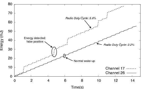
Figure 13: 802.11 b/g interference on the mote 802.15.4 radio. In the top curve the mote was set to the 802.15.4 channel 17, and in the bottom curve, to channel 26. These are, respectively, the closest to and furthest from the 802.11 b channel 6 which was used in the experiment.
We verified a significant impact of the interference: when on channel 17, the node falsely detected activity on the channel 17.8% of the time, had a radio duty cycle of 5.58±0.005%, and an average power draw of 1.43±0.08 mW. The nodes on channel 26, on the other hand, detected no false positives, had a duty cycle of 2.22±0.0027%, and an average power draw of 0.919±0.006 mW.
Figure 13 shows one measurement at each channel. The steps on the channel 17 curve are false positives, and have a marked effect on the cumulative energy consumption. Using Quanto, we estimated the current for the radio listen mode to be 18.46 mA, with a power draw of 61.8 mW (this particular mote was operating with a 3.35V switching regulator). Figure 14 shows two sampling events on channel 17. For both the radio and the CPU, the graph shows the power draw when active, and the respective activities. We can see the VTimer activity, which schedules the wake-ups, and the proxy receive activity, which doesn't get bound to any subsequent higher level activity. This is a simple example, but Quanto would be able to distinguish these activities even if the node were performing other tasks.
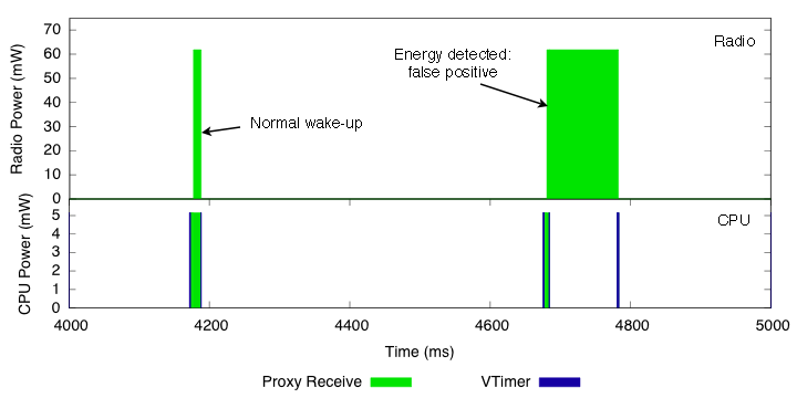
Figure 14: Detail of a normal wake-up period with no activity, in which the radio wakes up and returns to sleep, and of a false-positive activity detection. In the latter, the CPU keeps the radio on for about 100 ms, and turns it off when the timer expires and no packet was received.
Our second example concerns an effect we noticed when we instrumented a simple timer-based application on a single node. A particular timer interrupt, TimerA1, was firing repeatedly at 16Hz, as can be seen in Figure 15. This timer is used for calibrating a digital oscillator, which is not needed unless the node requires asynchronous serial communication. However, it was set to be always on, a behavior that surprised many of the TinyOS developers. The lack of visibility into the system made this behavior go unnoticed.
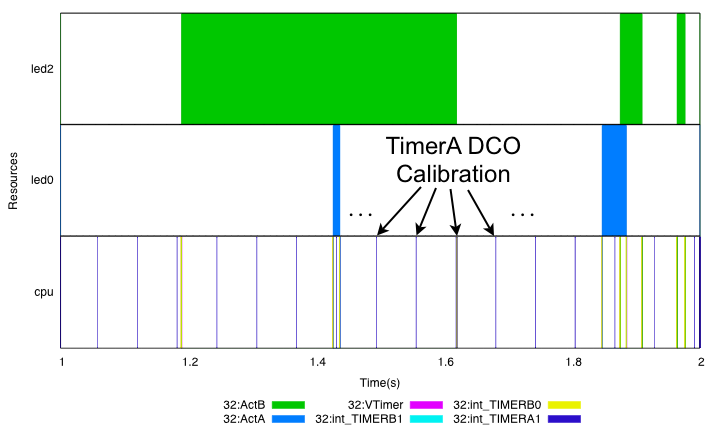
Figure 15: An unexpected result from instrumenting a simple application with Quanto: we noticed that a particular timer interrupt was firing 16 times per second for oscillator calibration, even when such calibration was unnecessary.
Our last example studies the effect of a particular setting of the radio stack: whether the CPU communicates with the radio chip using interrupts or a DMA channel. Figure 16 shows the timings captured by Quanto for a packet transmission, using both settings.
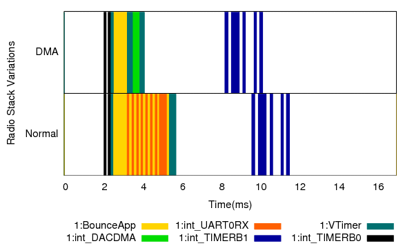
Figure 16: Timing behavior of a packet transmission using interrupt-driven and DMA-based communication between the CPU and the radio chip. Quanto allows the developer to understand the precise timing behavior of both options.
From the figure it is apparent that the DMA transfer is at least twice as fast as the interrupt-driven transfer. This has implications on how fast one can send packets, but more importantly, can influence the behavior of the MAC protocol. If two nodes A and B receive the same packet from a third node, and need to respond to it immediately, and if A uses DMA while B uses the interrupt-driven communication, A will gain access to the medium more often than B, subverting MAC fairness.
We now look at some of the costs associated with our prototype implementation of Quanto. These are summarized in Table 4.
The design of Quanto decouples generating event information, like activity and power state changes, from tracking the events. We currently record a log of the events for offline processing. The cost of logging is divided in two parts, one synchronous and one asynchronous. Recording the time and energy for each event has to be done synchronously, as close to the event as possible. Dealing with the recorded information can be done asynchronously.
It is very important to minimize the cost of synchronously recording each sample, as this both limits the rate at which we can capture successive events, and delays operations which must be processed quickly. Our current implementation records a 12-byte log entry for each event, described in Figure 17. We measured the cost of logging to RAM to be 101.7 µs, using the same technique as in [9]. At 1MHz, this translates to 102 cycles. This time includes 24 µs to read the iCount value, and 19 µs to read a timer value.
typedef struct entry_t {
  uint8_t type;     // type of the entry
  uint8_t res_id;   // hardware resource for entry
  uint32_t time;    // local time of the node
  uint32_t ic;      // icount: cumulative energy
  union {
    uint16_t act;         //for ctx changes
    uint16_t powerstate;  //for powerstate changes
  };
} entry_t;
Figure 17: The structure for the activity and powerstate log entry.
Because Quanto uses the CPU to keep track of state and to log changes to state, using it incurs a cost by delaying operations on the CPU, and spending more energy. For the run of Blink in Section 4.2, we logged 597 messages over 48 seconds. The total time spent on the logging itself was 60.71 ms, corresponding to 71.05% of the active CPU time, but only 0.12% of the total CPU time. The total energy spent with logging, assuming that logging is using the CPU and the Constant terms in the regression results, was 0.41 mJ, or 0.08% of the total energy spent. Although the 71% number is high, the majority of applications in these sensor network platforms strive to reduce the CPU duty cycle to save energy, and we expect the same trend of long idle periods to amortize the cost of logging.
The above numbers only concern the synchronous part. We still have to get the data out of the node for the current approach of offline analysis. We have two implementations for this. The first records messages to a fixed buffer in RAM that holds 800 log entries, periodically stops the logging, and dumps the information to the serial port or to the radio. The advangate of this is that the cost of logging, during the period being monitored, is only the cost of the synchronous part.
The second approach allows continuous logging. The processor still collects entries to the memory buffer, and schedules a low priority task to empty the log. This happens only when the CPU would otherwise be idle. Messages are written directly to an output port of the microprocessor, which drives an external synchronous serial interface. Like the Unix top application, Quanto can account for its own logging in this mode as its own activity. For the applications we instrumented, it used between 4 and 15% of the CPU time.
The rate of generated data from Quanto largely depends on the nature of the workload of the application. For the classes of applications that are common in embedded sensor networks, of low data-rate and duty cycle, we believe the overheads are acceptable.
Finally, we look at the burden to instrument a system like TinyOS to allow tracking and propagation of activities and power states. Table 5 lists the main abstractions we had to instrument in TinyOS to achieve propagation of activity labels in our platform, and shows that the changes are highly localized and relatively small in number of lines of code.
The complexity of the instrumentation task varies, and some device drivers with shadowed state that represents volatile state in peripherals can be more challenging to instrument. The CC2420 radio is a good example, as it has several internal power states and does some processing without the CPU intervention. Other devices, like the LEDs and simple sensors, are quite easier. We found that once the system is instrumented, the burden to the application programmer is small, since all that needs to be done is marking the beginning of relevant activities, which will be tracked and logged automatically.
Files Diff LOC Modified Code Tasks 2 25 Concurrency Timers 2 16 Deferral Arbiter 5 34 Locks Interrupts 11 88 Active Msg. 2 8 Link Layer LEDs 2 33 Device Driver CC2420 Radio 11 105 Device Driver SHT11 3 10 Sensor New code 28 1275 Infrastructure
Table 5: The cost of instrumenting most core primitives for activity and power tracking in TinyOS, as well as some representative device drivers, is low in terms of lines of code. New code represents the infrastructure code for keeping track of and logging activities and power states.
We now discuss some of the the design tradeoffs and limitations of the approach, and some research directions enabled by this work.
Logging vs. counting. Quanto currently logs every power state and activity context change which can result in large volume of trace data. The data are useful for reconstructing a fine-grained timeline and tracing causal connections, but this level of detail may be unnecessary in many cases. The design, however, clearly separates the event generation from the event consumption. An alternative would be to maintain a set counters on the nodes, accumulating time and energy spent per activity. In our initial exploration we decided to examine the full dataset offline, and leave as future work to explore performing the regression and accounting of resources online, which would make the memory overhead fixed and practically eliminate the logging overhead.
Activity model. An important design decision in Quanto is that activities are not hierarchical. While giving more flexibility, representing hierarchies would mean that the system would propagate stacks of activity labels instead of single labels, a significant increase in overhead and complexity. If a module C does work on behalf of two activities, A and B, the instrumenter has two options: to give C its own activity, or to have C's operations assume the activity of the caller.
Platform hardware support. All of the data in this paper were collected using the HydroWatch platform but our experiences suggested that a more tailored design would be useful. In particular, we had the options of storing the logs in RAM, which has little impact but limited space, or logging to a processor port, which has a slightly higher cost and can be intrusive at very high loads. We have designed a new platform tailored for profiling with a fast, 128 KB-deep FIFO for full speed logging with very little overhead, which we plan to use on future experiments.
Constant per-state power draws. The regression techniques used to estimate per-component energy usage assume the power draw of a hardware component is approximately constant in each power state. Fortunately, we verified that this assumption largely holds for the platform we instrumented, by looking at different length sampling intervals for each state. The regression may not work well when this assumption fails, but we leave quantifying this for future work.
Linear independence. The regression techniques also assume that tracking power states over time produces a set of linearly independent equations. If this is not the case, for example if unrelated actions always occur together, then regression is unlikely to disambiguate their energy usage. As a work around, custom routines can be written to exercise different power states independently.
Modifications to systems. Quanto requires the OS, including device drivers, and applications, to be modified to perform tracking. The modifications to the system, however, can be shared among all applications, and the modifications to applications are, in most cases, simple. Device drivers have to be modified so that they expose the power states of the underlying hardware components. If hardware power states are not observable, estimation errors may occur.
Energy usage visibility. Our approach may not generalize to systems with sophisticated power supply filtering (e.g. power factor correction or large capacitors) because these elements introduce a potentially non-linear phase delay between real and observed energy usage over short time scales, making it difficult to correlate short-lived activities with their energy usage.
Hardware energy metering. Our proposed approach requires hardware support for energy metering, which may not be available on some platforms. Fortunately, the energy meter design we use may be feasible on many systems that use pulse-frequency modulated switching regulators. However, even if hardware-based energy metering is not available, a software-based approach using hardware power models may still provide adequate visibility for some applications.
Finding energy leaks. A situation familiar to many developers is discovering that an application draws too much power but not knowing why. Using Quanto, developers can visualize energy usage over time by hardware component, allowing one to work backward to find the offending code that caused the energy leak.
Tracking butterfly effects. In many distributed applications, an action at one node can have network-wide effects. For example, advertising a new version of a code image or initiating a flood will cause significant network-wide action and energy usage. Even minor local actions, like a routing update, can ripple through the entire network. Quanto can trace the causal chain from small, local cause to large, network-wide effect.
Real time tracking. An extension of the framework can include performing the regression online, and replacing the logging with accumulators for time and energy usage per activity. This approach would have significantly reduced bandwidth and storage requirements, and could be used as an always on, network-wide energy profiler analogous to top.
Enery-Aware Scheduling. Since Quanto already tracks energy usage by activity, an extension to the operating system scheduler would enable energy-aware policies like equal-energy scheduling for threads, rather than equal-time scheduling.
Continuous Profiling. Quanto log entries are lightweight enough that continuous profiling is possible with even a modest speed logging back-channel [1].
Our techniques borrow heavily from the literature on energy-aware operating system, power simulation tools, power/energy metering, power profiling, resource containers, and distributed tracing.
ECOSystem [37] proposes the Currentcy model which treats energy as a first class resource that cuts across all existing system resources, such as CPU, disk, memory, and the network in a unified manner. Quanto leverages many of the ideas developed in ECOSystem, like tracking power states to allocate energy usage or employing resource containers as the principal to which resource usage is charged. But there are important differences as well. ECOSystem uses offline profiling to relate power state and power draw, and uses a model for runtime operation. In contrast, Quanto tracks the actual energy used at runtime, which is useful when environmental factors can affect energy availability and usage. While ECOSystem tracks energy usage on a single node, Quanto transparently tracks energy usage across the network, which allows network-wide effects to be measured. Finally, the focus of the two efforts is different although similar techniques are used in both systems.
Eon is a programming language and runtime system that allows paths or flows through the program to be annotated with different energy states [29]. Eon's runtime then chooses flows to execute, and their rates of execution, to maximize the quality of service under available energy constraints. Eon, like Quanto, uses real-time energy metering but attributes energy usage only to flows, while Quanto attributes usage to hardware, activity, and time.
Several power simulation tools exist that use empirically-generated models of hardware behavior. PowerTOSSIM [28] uses same-code simulation of TinyOS applications with power state tracking, combined with a power model of the different peripheral states, to create a log of energy usage. PowerTOSSIM provides visibility into the power draw based on its model of the hardware, but it does not capture the variability common in real hardware or operating environments, or simulate a device's interactions with the real world. Quanto also addresses a different problem than PowerTOSSIM: tracing the energy usage of logical activities rather than the time spent in software modules.
The challenge in taking measurements in low-power, embedded systems that exhibit bursty operation is that until recently, the performance of available metering options was simply too poor, and the power cost was simply too high, to use in actual deployments. Traditional instrument-based power measurements are useful for design-time laboratory testing but impractical for everyday run-time use due to the cost of instruments, their physical size, and their poor system integration [14, 12, 35]. Dedicated power metering hardware can enable run-time energy metering but they too come with the expense of increased hardware costs and power draws [5, 18]. Using hardware performance counters as a proxy power meter is possible on high-performance microprocessors like the Intel Pentium Pro [20] and embedded microprocessors like the Intel PXA255 [7]. Quanto addresses these challenges with iCount, a new design based on a switching regulator [9].
Of course, if a system employs only one switching regulator, then the energy usage can be measured only in the aggregate, rather than by hardware component. This aggregated view of energy usage can present some tracking challenges as well. One way to track the distinct power draws of the hardware components is to instrument their individual power supply lines [34, 30]. These approaches, however, are best suited to bench-scale investigations since they require extensive per-system calibration and the latter requires considerable additional hardware which would dominate the system power budget in our applications.
The Rialto operating system [19] introduced activities as the abstraction to which resources are allocated and charged. Resource Containers [2] use a similar notion, and acknowledge that there is a mismatch between traditional OS resource principals, namely threads and processes, and independent activities, especially in high performance network servers. Quanto borrows the concept of activities and extends them across all hardware components and across the nodes in a network.
Several previous works have modeled the behavior of distributed systems as a collection of causal paths including Magpie [3], Pinpoint [6], X-Trace [15], and Pip [27]. These systems reconstruct causal paths using some combinations of OS-level tracing, application-level annotation, and statistical inference. Causeway [4] instruments the FreeBSD OS to automatically carry metadata with the execution of threads and across machines. Quanto borrows from these earlier approaches and applies them to the problem of tracking network-wide energy usage in embedded systems, where resource constraints and energy consumption by hardware devices raise a number of different design tradeoffs.
The techniques developed and evaluated in this paper – breaking down the aggregate energy usage of a system by hardware component, tracking causally-connected energy usage of programmer-defined activities, and tracking the network-wide energy usage due to node-local actions – collectively provide visibility into when, where, and why energy is consumed both within a single node and across the network. Going forward, we believe this unprecedented visibility into energy usage will enable empirical evaluation of the energy-efficiency claims in the literature, provide ground truth for lightweight approximation techniques like counters, and enable energy-aware operating systems research.
This material is based upon work supported by the National Science Foundation under grants #0435454 (“NeTS-NR”) and #0454432 (“CNS-CRI”). This work was also supported by a National Science Foundation Graduate Research Fellowship and a Microsoft Research Graduate Fellowship as well as generous gifts from Hewlett-Packard Company, Intel Research, Microsoft Corporation, and Sharp Electronics.
This document was translated from LATEX by HEVEA.