cSamp: A System for Network-Wide Flow MonitoringVyas Sekar⋆, Michael
K. Reiter†, Walter
Willinger‡, Hui
Zhang⋆,
|
Critical network management applications increasingly demand fine-grained flow level measurements. However, current flow monitoring solutions are inadequate for many of these applications. In this paper, we present the design, implementation, and evaluation of cSamp, a system-wide approach for flow monitoring. The design of cSamp derives from three key ideas: flow sampling as a router primitive instead of uniform packet sampling; hash-based packet selection to achieve coordination without explicit communication; and a framework for distributing responsibilities across routers to achieve network-wide monitoring goals while respecting router resource constraints. We show that cSamp achieves much greater monitoring coverage, better use of router resources, and enhanced ability to satisfy network-wide flow monitoring goals compared to existing solutions.
Network operators routinely collect flow-level measurements to guide several network management applications. Traditionally, these measurements were used for customer accounting [9] and traffic engineering [13], which largely rely on aggregate traffic volume statistics. Today, however, flow monitoring assists several other critical network management tasks such as anomaly detection [19], identification of unwanted application traffic [6], and even forensic analysis [38], which need to identify and analyze as many distinct flows as possible. The main consequence of this trend is the increased need to obtain fine-grained flow measurements.
Yet, because of technological and resource constraints, modern routers cannot each record all packets or flows that pass through them. Instead, they rely on a variety of sampling techniques to selectively record as many packets as their CPU and memory resources allow. For example, most router vendors today implement uniform packet sampling (e.g., Netflow [5]); each router independently selects a packet with a sampling probability (typically between 0.001 and 0.01) and aggregates the selected packets into flow records. While sampling makes passive measurement technologically feasible (i.e., operate within the router constraints), the overall fidelity of flow-level measurements is reduced.
There is a fundamental disconnect between the increasing requirements of new network management applications and what current sampling techniques can provide. While router resources do scale with technological advances, it is unlikely that this disconnect will disappear entirely, as networks continue to scale as well. We observe that part of this disconnect stems from a router-centric view of current measurement solutions. In today's networks, routers record flow measurements completely independently of each other, thus leading to redundant flow measurements and inefficient use of router resources.
We argue that a centralized system that coordinates monitoring responsibilities across different routers can significantly increase the flow monitoring capabilities of a network. Moreover, such a centralized system simplifies the process of specifying and realizing network-wide flow measurement objectives. We describe Coordinated Sampling (cSamp), a system for coordinated flow monitoring within an Autonomous System (AS). cSamp treats a network of routers as a system to be managed in a coordinated fashion to achieve specific measurement objectives. Our system consists of three design primitives:
We address several practical aspects in the design and implementation of cSamp. We implement efficient algorithms for computing sampling manifests that scale to large tier-1 backbone networks with hundreds of routers. We provide practical solutions for handling multi-path routing and realistic changes in traffic patterns. We also implement a prototype using an off-the-shelf flow collection tool.
We demonstrate that cSamp is fast enough to respond in real time to realistic network dynamics. Using network-wide evaluations on the Emulab testbed, we also show that cSamp naturally balances the monitoring load across the network, thereby avoiding reporting hotspots. We evaluate the benefits of cSamp over a wide range of network topologies. cSamp observes more than twice as many flows compared with traditional uniform packet sampling, and is even more effective at achieving system-wide monitoring goals. For example, in the case of the minimum fractional flow coverage across all pairs of ingress-egress pairs, it provides significant improvement over other flow monitoring solutions. ISPs can derive several operational benefits from cSamp, as it reduces the reporting bandwidth and the data management overheads caused by duplicated flow reports. We also show that cSamp is robust with respect to errors in input data and realistic changes in traffic.
The design of cSamp as a centrally managed network-wide monitoring system is inspired by recent trends in network management. In particular, recent work has demonstrated the benefits of a network-wide approach for traffic engineering [13, 41] and network diagnosis [19, 20, 23]. Other recent proposals suggest that a centralized approach can significantly reduce management complexity and operating costs [1, 2, 14].
Despite the importance of network-wide flow monitoring, there have been few attempts in the past to design such systems. Most of the related work focuses on the single-router case and on providing incremental solutions to work around the limitations of uniform packet sampling. This includes work on adapting the packet sampling rate to changing traffic conditions [11, 17], tracking heavy-hitters [12], obtaining better traffic estimates from sampled measurements [9, 15], reducing the overall amount of measurement traffic [10], and data streaming algorithms for specific applications [18, 21].
Early work on network-wide monitoring has focused on the placement of monitors at appropriate locations to cover all routing paths using as few monitors as possible [4, 35]. The authors show that such a formulation is NP-hard, and propose greedy approximation algorithms. In contrast, cSamp assumes a given set of monitoring locations along with their resource constraints and, therefore, is complementary to these approaches.
There are extensions to the monitor-placement problem in [35] to incorporate packet sampling. Cantieni et al. also consider a similar problem [3]. While the constrained optimization formulation in these problems shares some structural similarity to our approach in Section 4.2, the specific contexts in which these formulations are applied are different. First, cSamp focuses on flow sampling as opposed to packet sampling. By using flow sampling, cSamp provides a generic flow measurement primitive that subsumes the specific traffic engineering applications that packet sampling (and the frameworks that rely on it) can support. Second, while it is reasonable to assume that the probability of a single packet being sampled multiple times across routers is negligible, this assumption is not valid in the context of flow-level monitoring. The probability of two routers sampling the same flow is high as flow sizes follow heavy-tailed distributions [7, 40]. Hence, cSamp uses mechanisms to coordinate routers to avoid duplicate flow reporting.
To reduce duplicate measurements, Sharma and Byers [33] suggest the use of Bloom filters. While minimizing redundant measurements is a common high-level theme between cSamp and their approach, our work differs on two significant fronts. First, cSamp allows network operators to directly specify and satisfy network-wide objectives, explicitly taking into account (possibly heterogeneous) resource constraints on routers, while their approach does not. Second, cSamp uses hash-based packet selection to implement coordination without explicit communication, while their approach requires every router to inform every other router about the set of flows it is monitoring.
Hash-based packet selection as a router-level primitive was suggested in Trajectory Sampling [8]. Trajectory Sampling assigns all routers in the network a common hash range. Each router in the network records the passage for all packets that fall in this common hash range. The recorded trajectories of the selected packets are then used for applications such as fault diagnosis. In contrast, cSamp uses hash-based selection to achieve the opposite functionality: it assigns disjoint hash ranges across multiple routers so that different routers monitor different flows.
Uniform Packet Data Streaming Heavy-hitter Flow sampling Flow sampling cSamp Sampling Algorithms monitoring (low-rate) (high-rate) (e.g. [3, 5]) (e.g., [18, 21]) (e.g., [12]) High flow coverage × × × × √ √ Avoiding redundant measurements × × × × × √ Network-wide flow monitoring goals × × × × × √ Operate within resource constraints √ √ √ √ × √ Generality to support many applications × × × × √ √
Table 1: Qualitative comparison across different deployment alternatives available to network operators.
We identify five criteria that a flow monitoring system should satisfy: (i) provide high flow coverage, (ii) minimize redundant reports, (iii) satisfy network-wide flow monitoring objectives (e.g., specifying some subsets of traffic as more important than others or ensuring fairness across different subsets of traffic), (iv) work within router resource constraints, and (v) be general enough to support a wide spectrum of flow monitoring applications. Table 1 shows a qualitative comparison of various flow monitoring solutions across these metrics.
Packet sampling implemented by routers today is inherently biased toward large flows, thus resulting in poor flow coverage. Thus, it does not satisfy the requirements of many classes of security applications [25]. In addition, this bias increases redundant flow reporting.
There exist solutions (e.g., [12, 18, 21]) that operate efficiently within router resource constraints, but either lack generality across applications or, in fact, reduce flow coverage. For example, techniques for tracking flows with high packet counts (e.g., [10, 12]) are attractive single-router solutions for customer accounting and traffic engineering. However, they increase redundant monitoring across routers without increasing flow coverage.
Flow sampling is better than other solutions in terms of flow coverage and avoiding bias toward large flows. However, there is an inherent tradeoff between the flow coverage and router resources such as reporting bandwidth and load. Also, flow sampling fails to achieve network-wide objectives with sufficient fidelity.
As Table 1 shows, none of the existing solutions simultaneously satisfy all the criteria. To do so, we depart from the router-centric approach adopted by existing solutions and take a more system-wide approach. In the next section, we describe how cSamp satisfies these goals by considering the routers in the network as a system to be managed in a coordinated fashion to achieve network-wide flow monitoring objectives.
In this section, we present the design of the hash-based flow sampling primitive and the optimization engine used in cSamp. In the following discussion, we assume the common 5-tuple (srcIP, dstIP, srcport, dstport, protocol) definition of an IP flow.
Hash-based flow sampling: Each router has a sampling manifest – a table of hash ranges indexed using a key. Upon receiving a packet, the router looks up the hash range using a key derived from the packet's header fields. It computes the hash of the packet's 5-tuple and samples the packet if the hash falls within the range obtained from the sampling manifest. In this case, the hash is used as an index into a table of flows that the router is currently monitoring. If the flow already exists in the table, it updates the byte and packet counters (and other statistics) for the flow. Otherwise it creates a new entry in the table.
The above approach implements flow sampling [15], since only those flows whose hash lies within the hash range are monitored. Essentially, we can treat the hash as a function that maps the input 5-tuple into a random value in the interval [0,1]. Thus, the size of each hash range determines the flow sampling rate of the router for each category of flows in the sampling manifest.
Flow sampling requires flow table lookups for each packet; the flow table, therefore, needs to be implemented in fast SRAM. Prior work has shown that maintaining counters in SRAM is feasible in many situations [12]. Even if flow counters in SRAM are not feasible, it is easy to add a packet sampling stage prior to flow sampling to make DRAM implementations possible [17]. For simplicity, however, we assume that the counters can fit in SRAM for the rest of the paper.
Coordination: If each router operates in isolation, i.e., independently sampling a subset of flows it observes, the resulting measurements from different routers are likely to contain duplicates. These duplicate measurements represent a waste of memory and reporting bandwidth on routers. In addition, processing duplicated flow reports incurs additional data management overheads.
Hash-based sampling enables a simple but powerful coordination strategy to avoid these duplicate measurements. Routers are configured to use the same hash function, but are assigned disjoint hash ranges so that the hash of any flow will match at most one router's hash range. The sets of flows sampled by different routers will therefore not overlap. Importantly, assigning non-overlapping hash ranges achieves coordination without explicit communication. Routers can thus achieve coordinated tasks without complex distributed protocols.
ISPs typically specify their network-wide goals in terms of Origin-Destination (OD) pairs, specified by the ingress and egress routers. To achieve flow monitoring goals specified in terms of OD-pairs, cSamp's optimization engine needs the traffic matrix (the number of flows per OD-pair) and routing information (the router-level path(s) per OD-pair), both of which are readily available to network operators [13, 41].
Assumptions and notation: We make two assumptions to simplify the discussion. First, we assume that the traffic matrix (number of IP flows per OD-pair) and routing information for the network are given exactly and that these change infrequently. Second, we assume that each OD-pair has a single router-level path. We relax these assumptions in Section 4.4 and Section 4.5.
Each OD-pair ODi (i = 1,…,M) is characterized by its router-level path Pi and the number Ti of IP flows in a measurement interval (e.g., five minutes).
Each router Rj (j = 1,…,N) is constrained by two resources: memory (per-flow counters in SRAM) and bandwidth (for reporting flow records). (Because we assume that the flow counters are stored in SRAM, we do not model packet processing constraints [12].) We abstract these into a single resource constraint Lj, the number of flows router Rj can record and report in a given measurement interval.
Let dij denote the fraction of the IP flows of ODi that router Rj samples. If Rj does not lie on path Pi, then the variable dij will not appear in the formulation. For i = 1,…,M, let Ci denote the fraction of flows on ODi that is monitored.
Objective: We present a general framework that is flexible enough to support several possible flow monitoring objectives specified as (weighted) combinations of the different Ci values. As a concrete objective, we consider a hybrid measurement objective that maximizes the total flow-coverage across all OD-pairs (∑iTi × Ci ) subject to ensuring the optimal minimum fractional coverage per OD-pair (mini {Ci}).
Problem maxtotgivenfrac(α):
|
|||||||||||||||||||||||||||||||||||||||||||||
We define a linear programming (LP) formulation that takes as a parameter α, the desired minimum fractional coverage per OD-pair. Given α, the LP maximizes the total flow coverage subject to ensuring that each OD-pair achieves a fractional coverage at least α, and that each router operates within its load constraint.
We briefly explain each of the constraints. (1) ensures that the number of flows that Rj is required to monitor does not exceed its resource constraint Lj. As we only consider sampling manifests in which the routers on Pi for ODi will monitor distinct flows, (2) says that the fraction of traffic of ODi that has been covered is simply the sum of the fractional coverages dij of the different routers on Pi. Because each Ci represents a fractional quantity we have the natural upper bound Ci ≤ 1 in (4). Since we want to guarantee that the fractional coverage on each OD-pair is greater than the desired minimum fractional coverage, we have the lower bound in (5). Since the dij define fractional coverages, they are constrained to be in the range [0,1]; however, the constraints in (4) subsume the upper bound on each dij and we impose the non-zero constraints in (3).
To maximize the total coverage subject to achieving the highest possible minimum fractional coverage, we use a two-step approach. First, we obtain the optimal minimum fractional coverage by considering the problem of maximizing mini {Ci} subject to constraints (1)–(4). Next, the value of OptMinFrac obtained from this optimization is used as the input α to maxtotgivenfrac.
The solution to the above two-step procedure, d* = ⟨ dij*⟩1 ≤ i ≤ M, 1 ≤ j ≤ N provides a sampling strategy that maximizes the total flow coverage subject to achieving the optimal minimum fractional coverage per OD-pair.
The next step is to map the optimal solution into a sampling manifest for each router that specifies its monitoring responsibilities (Figure 1). The algorithm iterates over the M OD-pairs. For each ODi, the variable Range is advanced in each iteration (i.e., per router) by the fractional coverage (dij*) provided by the current router (lines 4 and 5 in Figure 1). This ensures that routers on the path Pi for ODi are assigned disjoint ranges. Thus, no flows are monitored redundantly.
Once a router has received its sampling manifest, it implements the algorithm shown in Figure 2. For each packet it observes, the router first identifies the OD-pair. Next, it computes a hash on the flow headers (the IP 5-tuple) and checks if the hash value lies in the assigned hash range for the OD-pair (the function Hash returns a value in the range [0,1]). That is, the key used for looking up the hash range (c.f., Section 4.1) is the flow's OD-pair. Each router maintains a Flowtable of the set of flows it is currently monitoring. If the packet has been selected, then the router either creates a new entry (if none exists) or updates the counters for the corresponding entry in the Flowtable.
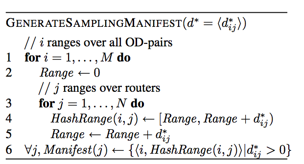
Figure 1: Translating the optimal solution into a sampling manifest for each router
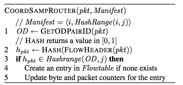
Figure 2: Algorithm to implement coordinated sampling on router Rj
The discussion so far assumed that the traffic matrices are known and fixed. Traffic matrices are typically obtained using estimation techniques (e.g., [41, 42]) that may have estimation errors.
If the estimation errors are bounded, we scale the sampling strategy appropriately to ensure that the new scaled solution will operate within the router resource constraints and be near-optimal in comparison to an optimal solution for the true (but unknown) traffic matrix.
Suppose the estimation errors in the traffic matrix are bounded, i.e., if Ti and Ti denote the estimated and actual traffic for ODi respectively, then ∀ i, Ti ∈ [ Ti(1−є), Ti(1+є) ]. Here, є quantifies how much the estimated traffic matrix (i.e., our input data) differs with respect to the true traffic matrix. Suppose the optimal sampling strategy for T = ⟨ Ti ⟩1 ≤ i ≤ M is d = ⟨ dij⟩1 ≤ i ≤ M, 1 ≤ j ≤ N, and that the optimal sampling strategy for T = ⟨ Ti ⟩1 ≤ i ≤ M is d* = ⟨ dij* ⟩1 ≤ i ≤ M, 1 ≤ j ≤ N.
A sampling strategy d is T-feasible if it satisfies conditions (1)–(4) for T. For a T-feasible strategy d, let β(d,T)= mini {Ci} denote the minimum fractional coverage, and let γ(d,T) = ∑i Ti × Ci = ∑i Ti × (∑j dij) denote the total flow coverage. Setting d'ij = dij* (1 − є), we can show that d' is T-feasible, and1
|
For example, with є = 1%, using d' yields a worst case performance reduction of 2% in the minimum fractional coverage and 4% in the total coverage with respect to the optimal strategy d.
Next, we discuss a practical extension to incorporate multiple paths per OD-pair, for example using equal cost multi-path routing (ECMP).2
Given the routing and topology information, we can obtain the multiple routing paths for each OD-pair and can compute the number of flows routed across each of the multiple paths. Then, we treat each of the different paths as a distinct logical OD-pair with different individual traffic demands. As an example, suppose ODi has two paths Pi1 and Pi2. We treat Pi1 and Pi2 as independent OD-pairs with traffic values Ti1 and Ti2. This means that we introduce additional dij variables in the formulation. In this example, in (1) we expand the term dij × Ti for router Rj to be dij1 × Ti1 + dij2 × Ti2 if Rj lies on both Pi1 and Pi2.
However, when we specify the objective function and the sampling manifests, we merge these logical OD-pairs. In the above example, we would specify the network-wide objectives in terms of the total coverage for the ODi, Ci = Ci1 + Ci2. This merging procedure also applies to the sampling manifests. For example, suppose Rj occurs on the two paths in the above example, and the optimal solution has values dij1 and dij2 corresponding to Pi1 and Pi2. The sampling manifest simply specifies that Rj is responsible for a total fraction dij = dij1 + dij2 of the flows in ODi.
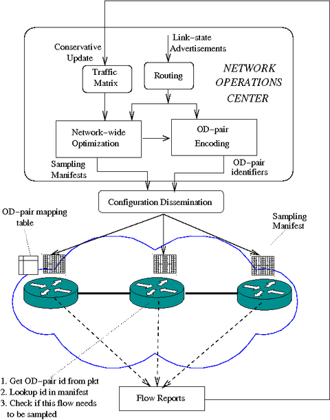
Figure 3: An overall view of the architecture of the cSamp system. The optimization engine uses up-to-date traffic and routing information to compute and disseminate sampling manifests to routers.
Figure 3 depicts the overall architecture of cSamp. The centralized optimization engine computes and disseminates sampling manifests based on the traffic matrix and routing information continuously measured in the network. This engine also assigns an identifier to every OD-pair and propagates this information to the ingress routers. The ingress routers determine the OD-pair and mark packets with the identifier. Each router uses the OD-pair identifier and its sampling manifest to decide if it should record a specific flow. In order to handle traffic dynamics, the optimization engine recalculates the traffic matrix periodically based on the observed flow reports to generate and distribute new sampling manifests. Such a centralized approach is consistent with the operating model of modern ISPs, where operators push out router configuration files (e.g., routing tables, ACLs) and collect information from the routers.
To complete the description of the cSamp system, we describe the following mechanisms: 1) obtaining OD-pair information for packets; 2) responding to long- and short-term traffic dynamics; 3) managing memory resources on routers; 4) computing the sampling manifests efficiently; and 5) reacting to routing dynamics.
Each router, on observing a packet, must identify the OD-pair to which the packet belongs. There are prior approaches to infer the OD-pair for a given packet based on the source and destination IP addresses and routing information [13]. However, such information may not be immediately discernible to interior routers from their routing tables due to prefix aggregation. Ingress routers are in a better position to identify the appropriate egress when a packet enters the network using such techniques. Thus the ingress routers mark each packet header with the OD-pair identifier. Interior routers can subsequently extract this information. In practice, the OD-pair identifier can either be added to the IP-header or to the MPLS label stack. Note that the multi-path extension (Section 4.5) does not impose additional work on the ingress routers for OD-pair identification. In both the single-path and multi-path cases, an ingress router only needs to determine the egress router and the identifier for the ingress-egress pair, and need not distinguish between the different paths for each ingress-egress pair.
The identifier can be added to the IP-id field in a manner similar to other proposals that rely on packet marking (e.g., [22, 29, 39]). This 16-bit field allows assigning a unique identifier to each OD-pair in a network with up to 256 border routers (and 65,536 OD-pairs), which suffices for medium-sized networks. For larger ISPs, we use an additional encoding step to assign identifiers to OD-pairs so that there are no conflicts in the assignments. For example, ODi and ODi' can be assigned the same identifier if Pi and Pi' do not traverse a common router (and the same interfaces on that router) or, if they do, the common router is not assigned logging responsibility for one of them. We formulate this notion of non-conflicting OD-pairs as a graph coloring problem, and run a greedy coloring algorithm on the resulting conflict graph. Using this extension, the approach scales to larger ISPs (e.g., needing fewer than 10 bits to encode all OD-pairs for a network with 300 border routers). In the interest of space, we do not discuss this technique or the encoding results further.
While the above approach to retrofit OD-pair identifiers within the IP header requires some work, it is easier to add the OD-pair identifier as a static label in the MPLS label stack. In this case, the space required to specify OD-pair identifiers is not a serious concern.
To ensure that the flow monitoring goals are achieved consistently over time, the optimization engine must be able to predict the traffic matrix to compute the sampling manifests. This prediction must take into account long-term variations in traffic matrices (e.g., diurnal trends), and also be able to respond to short-term dynamics (e.g., on the scale of a few minutes).
Long-term variations in traffic matrices typically arise from predictable time-of-day and day-of-week effects [28]. To handle these, we use historical traffic matrices as inputs to the optimization engine to compute the sampling strategy. For example, to compute the manifests for this week's Fri. 9am-10am period, we use the traffic matrix observed during the previous week's Fri. 9am-10am period.
The optimization engine also has to respond to less predictable short-term traffic variations. Using historical traffic matrices averaged over long periods (e.g., one week) runs the risk of underfitting; important structure present over shorter time scales is lost due to averaging. On the other hand, using historical traffic matrices over short periods (e.g., 5-minute intervals) may result in overfitting, unnecessarily incorporating details specific to the particular historical period in question.
To handle the long and short-term traffic dynamics, we take the following heuristic approach. Suppose we are interested in computing sampling manifests for every 5-minute interval for the Fri. 9am-10am period of the current week. To avoid overfitting, we do not use the traffic matrices observed during the corresponding 5-minute intervals that make up the previous week's Fri. 9am-10am period. Instead, we take the (hourly) traffic matrix for the previous week's Fri. 9am-10am period, divide it by 12 (the number of 5-minute segments per hour), and use the resulting traffic matrix Told as input data for computing the manifests for the first 5-minute period. At the end of this period, we collect flow data from each router and obtain the traffic matrix Tobs from the collected flow reports. (If the fractional coverage for ODi with the current sampling strategy is Ci and xi sampled flows are reported, then Tiobs = xi/Ci, i.e., normalizing the number of sampled flows by the total flow sampling rate.)
Given the observed traffic matrix for the current measurement period Tobs and the historical traffic matrix Told, a new traffic matrix is computed using a conservative update policy. The resulting traffic matrix Tnew is used as the input for obtaining the manifests for the next 5-minute period.
The conservative update policy works as follows. First, check if there are significant differences between the observed traffic matrix Tobs and the historical input data Told. Let δi = |Tiobs − Tiold|/Tiold denote the estimation error for ODi. If δi exceeds a threshold Δ, then compute a new traffic matrix entry Tinew, otherwise use Tiold. If Tiobs is greater than Tiold, then set Tinew = Tiobs. If Tiobs is smaller than Tiold, check the resource utilization of the routers currently responsible for monitoring ODi. If all these routers have residual resources available, set Tinew = Tiobs; otherwise set Tinew = Tiold.
The rationale behind this conservative update heuristic is that if a router runs out of resources, it may result in underestimating the new traffic on OD-pairs for which it is responsible (i.e., Tobs is an under-estimate of the actual traffic matrix). Updating Tnew with Tobs for such OD-pairs is likely to cause a recurrence of the same overflow condition in the next 5-minute period. Instead, we err on the side of overestimating the traffic for each OD-pair. This ensures that the information obtained for the next period is reliable and can help make a better decision when computing manifests for subsequent intervals.
The only caveat is that this policy may provide lower flow coverage since it overestimates the total traffic volume. Our evaluations with real traffic traces (Section 6.3) show that this performance penalty is low and the heuristic provides near-optimal traffic coverage.
We assume that the flow table is maintained in (more expensive) SRAM. Thus, we need a compact representation of the flow record in memory, unlike Netflow [5] which maintains a 64-byte flow record in DRAM. We observe that the entire flow record (the IP 5-tuple, the OD-pair identifier, and counters) need not actually be maintained in SRAM; only the flow counters (for byte and packet counts) need to be in SRAM. Thus, we can offload most of the flow fields to DRAM and retain only those relevant to the online computation: a four byte flow-hash (for flowtable lookups) and 32-bit counters for packets and bytes, requiring only 12 bytes of SRAM per flow record. To further reduce the SRAM required, we can use techniques for maintaining counters using a combination of SRAM and DRAM [43]. We defer a discussion of handling router memory exhaustion to Section 7.
In order to respond in near-real time to network dynamics, computing and disseminating the sampling manifests should require at most a few seconds. Unfortunately, the simple two-step approach in Section 4.2 requires a few hundreds of seconds on large ISP topologies and thus does not scale. We discovered that its bottleneck is the first step of solving the modified LP to find OptMinFrac.
To reduce the computation time we implement two optimizations. First, we use a binary search procedure to determine OptMinFrac. This was based on experimental evidence that solving the LP specified by maxtotgivenfrac(α) for a given α is faster than solving the LP to find OptMinFrac. Second, we use the insight that maxtotgivenfrac(α) can be formulated as a special instance of a MaxFlow problem. These optimizations reduce the time needed to compute the optimal sampling strategy to at most eleven seconds even on large tier-1 ISPs with more than 300 routers.
Binary search: The main idea is to use a binary search procedure over the value of α using the LP formulation maxtotgivenfrac(α). The procedure takes as input an error parameter є and returns a feasible solution with a minimum fractional coverage α* with the guarantee that OptMinFrac − α* ≤ є. The search keeps track of αlower, the smallest feasible value known (initially set to zero), and αupper, the highest possible value (initially set to ∑j Lj/∑i Ti). In each iteration, the lower and upper bounds are updated depending on whether the current value α is feasible or not and the current value α is updated to αlower+αupper/2. The search starts from α = αupper, and stops if the gap αupper − αlower is less than є, and returns α* = αlower at this stopping point.
Reformulation using MaxFlow: We formulate the LP maxtotgivenfrac(α) as an equivalent MaxFlow problem, specifically a variant of traditional MaxFlow problems that has additional lower-bound constraints on edge capacities. The intuition behind this optimization is that MaxFlow problems are typically more efficient to solve than general LPs.
We construct the following (directed) graph G = ⟨ V,E ⟩. The set of vertices in G is
| V = {source,sink} ⋃ { odi }1 ≤ i ≤ M ⋃ { rj}1 ≤ j ≤ N |
Each odi in the above graph corresponds to OD-pair ODi in the network and each rj in the graph corresponds to router Rj in the network.
The set of edges is E = E1 ∪ E2 ∪ E3, where
|
Let f(x,y) denote the flow on the edge (x,y) ∈ E, and let UB(x,y) and LB(x,y) denote the upper-bound and lower-bound on edge capacities in G. Our objective is to maximize the flow F from source to sink subject to the following constraints.
| ∀ x, | ⎛ ⎜ ⎜ ⎝ |
|
f(x,y) − |
|
f(y,x) | ⎞ ⎟ ⎟ ⎠ |
= | ⎧ ⎪ ⎨ ⎪ ⎩ |
|
We specify lower and upper bounds on the flow on each edge as:
| ∀ x, ∀ y, LB(x,y) ≤ f(x,y) ≤ UB(x,y) |
The upper-bounds on the edge capacities are: (i) the edges from the source to odi have a maximum capacity equal to Ti (the traffic for OD-pair ODi), and (ii) the edges from each rj to the sink have a maximum capacity equal to Lj (resource available on each router Rj).
| UB((x,y)) = | ⎧ ⎪ ⎨ ⎪ ⎩ |
|
We introduce lower bounds only on the edges from the source to each odi, indicating that each ODi should have a fractional flow coverage at least α:
| LB((x,y) ) = | ⎧ ⎨ ⎩ |
|
We use the binary search procedure discussed earlier, but use this MaxFlow formulation to solve each iteration of the binary search instead of the LP formulation.
The cSamp system receives real-time routing updates from a passive routing and topology monitor such as OSPF monitor [32]. Ideally, the optimization engine would recompute the sampling manifests for each routing update. However, recomputing and disseminating sampling manifests to all routers for each routing update is expensive. Instead, the optimization engine uses a snapshot of the routing and topology information at the beginning of every measurement interval to compute and disseminate manifests for the next interval. This ensures that all topology changes are handled within at most two measurement intervals.
To respond more quickly to routing changes, the optimization engine can precompute sampling manifests for different failure scenarios in a given measurement cycle. Thus, if a routing change occurs, an appropriate sampling manifest corresponding to this scenario is already available. This precomputation reduces the latency of adapting to a given routing change to less than one measurement interval. Since it takes only a few seconds (e.g., 7 seconds for 300 routers and 60,000 OD-pairs) to compute a manifest on one CPU (Section 6.1), we can precompute manifests for all single router/link failure scenarios with a moderate (4-5×) level of parallelism. While precomputing manifests for multiple failure scenarios is difficult, such scenarios are also relatively rare.
Optimization engine: Our implementation of the algorithms for computing sampling manifests (Section 5.4) consists of 1500 lines of C/C++ code using the CPLEX callable library. The implementation is optimized for repeated computations with small changes to the input parameters, in that it carries state from one solution over to the next. Solvers like CPLEX typically reach a solution more quickly when starting “close” to a solution than when starting from scratch. Moreover, the solutions that result tend to have fewer changes to the preceding solutions than would solutions computed from scratch, which enables reconfigured manifests to be deployed with fewer or smaller messages. We implement this optimization for both our binary search algorithm and when recomputing sampling manifests in response to traffic and routing dynamics.
Flow collection: We implemented a cSamp extension to the YAF flow collection tool.3 Our choice was motivated by our familiarity with YAF, its simplicity of implementation, and because it is a reference implementation for the IETF IPFIX working group. The extensions to YAF required 200 lines of additional code. The small code modification suggests that many current flow monitoring tools can be easily extended to realize the benefits of cSamp. In our implementation, we use the BOB hash function recommended by Molina et al. [26].
We divide our evaluation into three parts. First, we demonstrate that the centralized optimization engine and the individual flow collection processes in cSamp are scalable in Section 6.1. Second, we show the practical benefits that network operators can derive from cSamp in Section 6.2. Finally, in Section 6.3, we show that the system can effectively handle realistic traffic dynamics.
In our experiments, we compare the performance of different sampling algorithms at a PoP-level granularity, i.e., treating each PoP as a “router” in the network model. We use PoP-level network topologies from educational backbones (Internet2 and GÉANT) and tier-1 ISP backbone topologies inferred by Rocketfuel [34]. We construct OD-pairs by considering all possible pairs of PoPs and use shortest-path routing to compute the PoP-level path per OD-pair. To obtain the shortest paths, we use publicly available static IS-IS weights for Internet2 and GÉANT and inferred link weights [24] for Rocketfuel-based topologies.
Topology (AS#) PoPs OD-pairs Flows Packets × 106 × 106 NTT (2914) 70 4900 51 204 Level3 (3356) 63 3969 46 196 Sprint (1239) 52 2704 37 148 Telstra (1221) 44 1936 32 128 Tiscali (3257) 41 1681 32 218 GÉANT 22 484 16 64 Internet2 11 121 8 32
Table 2: Parameters for the experiments
Due to the lack of publicly available traffic matrices and aggregate traffic estimates for commercial ISPs, we take the following approach. We use a baseline traffic volume of 8 million IP flows for Internet2 (per 5-minute interval).4 For other topologies, we scale the total traffic by the number of PoPs in the topology (e.g., given that Internet2 has 11 PoPs, for Sprint with 52 PoPs the traffic is 52/11 × 8 = 37 million flows). These values match reasonably well with traffic estimates reported for tier-1 ISPs. To model the structure of the traffic matrix, we first annotate PoP k with the population pk of the city to which it is mapped. We then use a gravity model to obtain the traffic volume for each OD-pair [33]. In particular, we assume that the total traffic between PoPs k and k' is proportional to pk × pk'. We assume that flow size (number of packets) is Pareto-distributed, i.e., Pr(Flowsize > x packets)=(c/x)γ,x≥ c with γ=1.8 and c=4. (We use these as representative values; our results are similar across a range of flow size parameters.) Table 2 summarizes our evaluation setup.
In this section, we measure the performance of cSamp along two dimensions – the cost of computing sampling manifests and the router overhead.
AS PoP-level (secs) Router-level (secs) Bin-LP Bin-MaxFlow Bin-LP Bin-MaxFlow NTT 0.53 0.16 44.5 10.9 Level3 0.27 0.10 24.6 7.1 Sprint 0.01 0.08 17.9 4.8 Telstra 0.09 0.03 9.6 2.2 Tiscali 0.11 0.03 9.4 2.2 GÉANT 0.03 0.01 2.3 0.3 Internet2 0.01 0.005 0.20 0.14
Table 3: Time (in seconds) to compute the optimal sampling manifest for both PoP- and router-level topologies. Bin-LP refers to the binary search procedure without the MaxFlow optimization.
Computing sampling manifests: Table 3 shows the time taken to compute the sampling manifests on an Intel Xeon 2.80 GHz CPU machine for different topologies. For every PoP-level topology we considered, our optimization framework generates sampling manifests within one second, even with the basic LP formulation. Using the MaxFlow formulation reduces this further. On the largest PoP-level topology, NTT, with 70 PoPs, it takes only 160 ms to compute the sampling manifests with this optimization.
We also consider augmented router-level topologies constructed from PoP-level topologies by assuming that each PoP has four edge routers and one core router, with router-level OD-pairs between every pair of edge routers. To obtain the router-level traffic matrix, we split the inter-PoP traffic uniformly across the router-level OD-pairs constituting each PoP-level OD-pair.
Even with 5× as many routers and 16× as many OD-pairs as the PoP-level topologies, the worst case computation time is less than 11 seconds with the MaxFlow optimization. These results show that cSamp can respond to network dynamics in near real-time, and that the optimization step is not a bottleneck.
Worst-case processing overhead: cSamp imposes extra processing overhead per router to look up the OD-pair identifier in a sampling manifest and to compute a hash over the packet header. To quantify this overhead, we compare the throughput (on multiple offline packet traces) of running YAF in full flow capture mode, and running YAF with cSamp configured to log every flow. Note that this configuration demonstrates the worst-case overhead because, in real deployments, a cSamp instance would need to compute hashes only for packets belonging to OD-pairs that have been assigned to it, and update flow counters only for the packets it has selected. Even with this worst-case configuration the overhead of cSamp is only 5% (not shown).
Network-wide evaluation using Emulab: We use Emulab [37] for a realistic network-wide evaluation of our prototype implementation. The test framework consists of support code that (a) sets up network topologies; (b) configures and runs YAF instances per “router”; (c) generates offline packet traces for a given traffic matrix; and (d) runs real-time tests using the BitTwist5 packet replay engine with minor modifications. The only difference between the design in Section 4 and our Emulab setup is with respect to node configurations. In Section 4, sampling manifests are computed on a per-router basis, but YAF processes are instantiated on a per-interface basis. We map router-level manifests to interface-level manifests by assigning each router's responsibilities across its ingress interfaces. For example, if Rj is assigned the responsibility to log ODi, then this responsibility is assigned to the YAF process instantiated on the ingress interface for Pi on Rj.
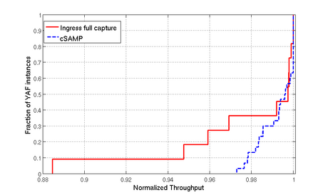
We configure cSamp in full-coverage mode, i.e., configured to capture all flows in the network (in our formulation this means setting the router resources such that OptMinFrac = 1). We also consider the alternative full coverage solution where each ingress router is configured to capture all traffic on incoming interfaces. The metric we compare is the normalized throughput of each YAF instance running in the emulated network. Let the total number of packets sent through the interface (in a fixed interval of 300 seconds) on which the YAF process is instantiated be pktsactual. Suppose the YAF instance was able to process only pktsprocessed packets in the same time interval. Then the normalized throughput is defined as pktsprocessed/pktsactual. By definition, the normalized throughput can be at most 1.
Our test setup is unfair to cSamp for two reasons. First, with a PoP-level topology, every ingress router is also a core router. Thus, there are no interior routers on which the monitoring load can be distributed. Second, to emulate a router processing packets on each interface, we instantiate multiple YAF processes on a single-CPU Emulab pc3000 node. In contrast, ingress flow capture needs exactly one process per Emulab node. In reality, this processing would be either parallelized in hardware (offloaded to individual linecards), or on multiple CPUs per YAF process even in software implementations, or across multiple routers in router-level topologies.
Figure 4 shows the distribution of the normalized throughput values of each YAF instance in the emulated network. Despite the disadvantageous setup, the normalized packet processing throughput of cSamp is higher. Given the 5% overhead due to hash computations mentioned before, this result might appear surprising. The better throughput of cSamp is due to two reasons. First, each per-interface YAF instance incurs per-packet flow processing overheads (look up flowtable, update counters, etc.) only for the subset of flows assigned to it. Second, we implement a minor optimization that first checks whether the OD-pair (identified from IP-id field) for the packet is present in its sampling manifest, and computes a hash only if there is an entry for this OD-pair. We also repeated the experiment by doubling the total traffic volume, i.e., using 16 million flows instead of 8 million flows. The difference between the normalized throughputs is similar in this case as well. For example, the minimum throughput with ingress flow capture is only 85%, whereas for cSamp the minimum normalized throughput is 93% (not shown). These results show that by distributing responsibilities across the network, cSamp balances the monitoring load effectively.
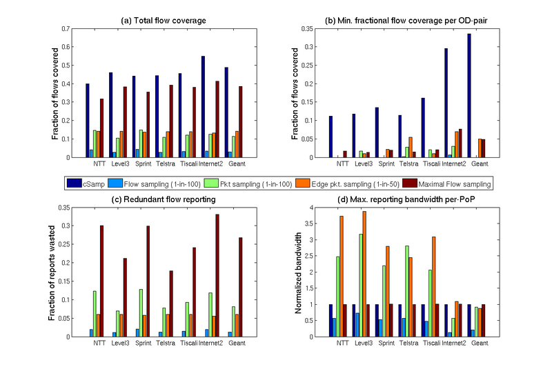
Figure 5: Comparing cSamp with packet sampling and hypothetical flow sampling approaches
It is difficult to scale our evaluations to larger topologies using Emulab. Therefore, we implemented a custom packet-level network simulator (roughly 2500 lines of C++) to evaluate the performance of different sampling approaches. For all the sampling algorithms, the simulator uses the same network topology, OD traffic matrix, and IP flow-size distribution for consistent comparisons.
We consider two packet sampling alternatives: (i) uniform packet sampling with a sampling rate of 1-in-100 packets at all routers in the network, and (ii) uniform packet sampling at edge routers (this may reflect a feasible alternative for some ISPs [13]) with a packet sampling rate of 1-in-50 packets. We also consider two flow sampling variants: (iii) constant-rate flow sampling at all routers with a sampling rate of 1-in-100 flows, and (iv) maximal flow sampling in which the flow sampling rates are chosen such that each node maximally utilizes its available memory. In maximal flow sampling, the flow sampling rate for a router is min(1,l/t), where l is the number of flow records it is provisioned to hold and t is the total number of flows it observes. Both constant-rate and maximal flow sampling alternatives are hypothetical; there are no implementations of either available in routers today. We consider them along with cSamp to evaluate different intermediate solutions in the overall design space, with current packet sampling approaches at one end of the spectrum and cSamp at the other. The metrics we consider directly represent the criteria in Table 1.
cSamp and the two flow sampling alternatives are constrained by the amount of SRAM on each router. We assume that each PoP in the network is provisioned to hold up to 400,000 flow records. Assuming roughly 5 routers per PoP, 10 interfaces per router, and 12 bytes per flow record, this requirement translates into 400,000 × 12/5 * 10 = 96 KB SRAM per linecard, which is well within the 8 MB technology limit (in 2004) suggested by Varghese [36]. (The total SRAM per linecard is shared across multiple router functions, but it is reasonable to allocate 1% of the SRAM for flow monitoring.) Since packet sampling alternatives primarily operate in DRAM, we use the methodology suggested by Estan and Varghese [12] and impose no memory restrictions on the routers. By assuming that packet sampling operates under no memory constraints, we provide it the best possible flow coverage (i.e., we underestimate the benefits of cSamp).
Coverage benefits: Figure 5(a) compares the total flow coverage obtained with different sampling schemes for the various PoP-level topologies (Table 2). The total flow coverage of cSamp is 1.8-3.3× that of the uniform packet sampling approaches for all the topologies considered. Doubling the sampling rate for edge-based uniform packet sampling only marginally improves flow coverage over all-router uniform packet sampling. Among the two flow sampling alternatives, constant rate flow sampling uses the available memory resources inefficiently, and the flow coverage is 9-16× less than cSamp. Maximal flow sampling uses the memory resources maximally, and therefore is the closest in performance. Even in this case, cSamp provides 14-32% better flow coverage. While this represents only a modest gain over maximal flow sampling, Figures 5(b) and 5(c) show that maximal flow sampling suffers from poor minimum fractional coverage and increases the amount of redundancy in flow reporting.
Figure 5(b) compares the minimum fractional coverage per OD-pair. cSamp significantly outperforms all alternatives, including maximal flow sampling. This result shows a key strength of cSamp to achieve network-wide flow coverage objectives, which other alternatives fail to provide. In addition, the different topologies vary significantly in the minimum fractional coverage, in comparison to the total coverage. For example, the minimum fractional coverage for Internet2 and GÉANT is significantly higher than other ASes even though the traffic volumes in our simulations are scaled linearly with the number of PoPs. We attribute this to the unusually large diagonal and near-diagonal elements in a traffic matrix. For example, in the case of Telstra, the bias in the population distribution across PoPs is such that the top few densely populated PoPs (Sydney, Melbourne, and Los Angeles) account for more than 60% of the total traffic in the gravity-model based traffic matrix.
Reporting benefits: In Figure 5(c), we show the ratio of the number of duplicate flow records reported to the total number of distinct flow reports reported. The absence of cSamp in Figure 5(c) is because of the assignment of non-overlapping hash-ranges to avoid duplicate monitoring. Constant rate flow sampling has little duplication, but it provides very low flow coverage. Uniform packet sampling can result in up to 14% duplicate reports. Edge-based packet sampling can alleviate this waste to some extent by avoiding redundant reporting from transit routers. Maximal flow sampling incurs the largest amount of duplicate flow reports (as high as 33%).
Figure 5(d) shows the maximum reporting bandwidth across all PoPs. We normalize the reporting bandwidth by the bandwidth required for cSamp. The reporting bandwidth for cSamp and flow sampling is bounded by the amount of memory that the routers are provisioned with; memory relates directly to the number of flow-records that a router needs to export. The normalized load for uniform packet sampling can be as high as four. Thus cSamp has the added benefit of avoiding reporting hotspots unlike traditional packet sampling approaches.
Summary of benefits: cSamp significantly outperforms traditional packet sampling approaches on all four metrics. Unlike constant rate flow sampling, cSamp efficiently leverages the available memory resources. While maximal flow sampling can partially realize the benefits in terms of total flow coverage, it has poor performance with respect to the minimum fractional flow coverage and the number of duplicated flow reports. Also, as network operators provision routers to obtain greater flow coverage, this bandwidth overhead due to duplicate flow reports will increase.
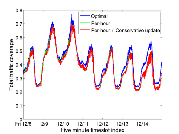
To evaluate the robustness of our approach to realistic traffic changes, we consider a two-week snapshot (Dec 1–14, 2006) of (packet sampled) flow data from Internet2. We map each flow entry to the corresponding network ingress and egress points using the technique outlined by Feldmann et al. [13].6 We assume that there are no routing changes in the network, and that the sampled flow records represent the actual traffic in the network. (Since cSamp does not suffer from flow size biases there is no need to renormalize the flow sizes by the packet sampling rate.) For this evaluation, we scale down the per-PoP memory to 50,000 flow records. (Due to packet sampling, the dataset contains fewer unique flows than the estimate in Table 2.)
Figure 6 compares the total flow coverage using our approach for handling traffic dynamics (Section 5.2) with the optimal total flow coverage (i.e., if we use the actual traffic matrix instead of the estimated traffic matrix to compute manifests). As expected, the optimal flow coverage exhibits time-of-day and day-of-week effects. For example, during the weekend, the coverage is around 70% while on the weekdays the coverage is typically in the 20-50% range. The result confirms that relying on traffic matrices that are based on hourly averages from the previous week gives near-optimal total flow coverage and represents a time scale of practical interest that avoids both overfitting and underfitting (Section 5.2). Using more coarse-grained historical information (e.g., daily or weekly averages) gives sub-optimal coverage (not shown). Figure 6 also shows that even though the conservative update heuristic (Section 5.2) overestimates the traffic matrix, the performance penalty arising from this overestimation is negligible.
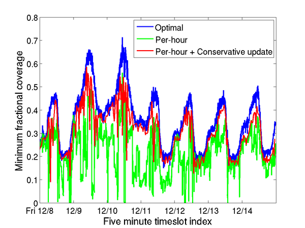
Figure 7 shows that using the per-hour historical estimates alone performs poorly compared to the optimal minimum fractional coverage. This is primarily because of short-term variations that the historical traffic matrices cannot account for. The conservative update heuristic significantly improves the performance in this case and achieves near-optimal performance. These results demonstrate that our approach of using per-hour historical traffic matrices combined with a conservative update heuristic is robust to realistic traffic dynamics.
Reliance on OD-pair identifiers: A key limitation of our design is the reliance on OD-pair identifiers. This imposes two requirements: (i) modifications to packet headers, and (ii) upgrades to border routers to compute the egress router [13] for each packet. While this assumption simplifies our design, an interesting question is whether it is possible to realize the benefits of a cSamp-like framework even when routers' sampling decisions are based only on local information.
Router memory exhaustion: Despite factoring in the router memory constraints into the optimization framework, a router's flow memory might be exhausted due to traffic dynamics. In our current prototype, we choose not to evict flow records already in the flow memory, but instead stop creating new flow records until the end of the measurement cycle. The conservative update heuristic (Section 5.2) will ensure that the traffic demands for the particular OD-pairs that caused the discrepancy are updated appropriately in the next measurement cycle.
In general, however, more sophisticated eviction strategies might be required to prevent unfairness within a given measurement cycle under adversarial traffic conditions. For example, one such strategy could be to allocate the available flow memory across all OD-pairs in proportion to their hash ranges and evict flows only from those OD-pairs that exceed their allotted share. While this approach appears plausible at first glance, it has the side effect that traffic matrices will not be updated properly to reflect traffic dynamics. Thus, it is important to jointly devise the eviction and the traffic matrix update strategies to prevent short-term unfairness, handle potential adversarial traffic conditions, and minimize the error in estimating traffic matrices. We intend to pursue such strategies as part of future work.
Transient conditions inducing loss of flow coverage or duplication: A loss in flow coverage can occur if a router that has been assigned a hash range for an OD-pair no longer sees any traffic for that OD-pair due to a routing change. Routing changes will not cause any duplication if the OD-pair identifiers are globally unique. However, if we encode OD-pair identifiers without unique assignments (see Section 5.1), then routing changes could result in duplication due to OD-pair identifier aliasing. Also, due to differences in the time for new configurations to be disseminated to different routers, there is a small amount of time during which routers may be in inconsistent sampling configurations resulting in some duplication or loss.
Applications of cSamp: cSamp provides an efficient flow monitoring infrastructure that can aid and enable many new traffic monitoring applications (e.g., [6, 16, 19, 30, 38]). As an example application that can benefit from better flow coverage, we explored the possibility of uncovering botnet-like communication structure in the network [27]. We use flow-level data from Internet2 and inject 1,000 synthetically crafted single-packet flows into the original trace, simulating botnet command-and-control traffic. cSamp uncovers 12× (on average) more botnet flows compared to uniform packet sampling. We also confirmed that cSamp provides comparable or better fidelity compared to uniform packet sampling for traditional traffic engineering applications such as traffic matrix estimation.
Flow-level monitoring is an integral part of the suite of network management applications used by network operators today. Existing solutions, however, focus on incrementally improving single-router sampling algorithms and fail to meet the increasing demands for fine-grained flow-level measurements. To meet these growing demands, we argue the need for a system-wide rather than router-centric approach for flow monitoring.
We presented cSamp, a system that takes a network-wide approach to flow monitoring. Compared to current solutions, cSamp provides higher flow coverage, achieves fine-grained network-wide flow coverage goals, efficiently leverages available monitoring capacity and minimizes redundant measurements, and naturally load balances responsibilities to avoid hotspots. We also demonstrated that our system is practical: it scales to large tier-1 backbone networks, it is robust to realistic network dynamics, and it provides a flexible framework to accommodate complex policies and objectives.
We thank Daniel Golovin for suggesting the scaling argument used in Section 4.4, Vineet Goyal and Anupam Gupta for insightful discussions on algorithmic issues, and Steve Gribble for shepherding the final version of the paper. This work was supported in part by NSF awards CNS-0326472, CNS-0433540, CNS-0619525, and ANI-0331653. Ramana Kompella thanks Cisco Systems for their support.
This document was translated from LATEX by HEVEA.