SRIKANTH KANDULA
KATE CHING-JU LIN
TURAL BADIRKHANLI
DINA KATABI
MIT
NTU/MIT
MIT
MIT
KANDULA@MIT.EDU
KATE@CSAIL.MIT.EDU
TURALB@MIT.EDU
DK@MIT.EDU
Abstract- It is increasingly common that computers in residential and hotspot scenarios see multiple access points (APs). These APs often provide high speed wireless connectivity but access the Internet via independent, relatively low-speed DSL or cable modem links. Ideally, a client would simultaneously use all accessible APs and obtain the sum of their backhaul bandwidth. Past work can connect to multiple APs, but can neither aggregate AP backhaul bandwidth nor can it maintain concurrent TCPs across them.
This paper introduces FatVAP, an 802.11 driver that aggregates the
bandwidth available at accessible APs and also balances their
loads. FatVAP has three key features. First, it chooses the APs that
are worth connecting to and connects with each AP just long enough to
collect its available bandwidth. Second, it ensures fast switching
between APs without losing queued packets, and hence is the only
driver that can sustain concurrent high throughput TCP connections
across multiple APs. Third, it works with unmodified APs and is
transparent to applications and the rest of the network stack. We
experiment with FatVAP both in our lab and hotspots and residential
deployments. Our results show that, in today's deployments, FatVAP
immediately delivers to the end user a median throughput gain of
![]() x, and reduces the median response time by
x, and reduces the median response time by ![]() x.
x.
Ideally, one would like a connectivity model that approximates a fat virtual AP, whose backhaul capacity is the sum of the access capacities of nearby APs. Users then compete fairly for this fat AP, limited only by security restrictions. A fat AP design benefits users because it enables them to harness unused bandwidth at accessible APs to maximize their throughput. It also benefits AP owners because load from users in a campus, office, or hotel is balanced across all nearby APs, reducing the need to install more APs.
It might seem that the right strategy to obtain a fat virtual AP would be to greedily connect to every AP. However, using all APs may not be appropriate because of the overhead of switching between APs. In fact, if we have to ensure that TCP connections simultaneously active across multiple APs do not suffer timeouts, it might be impossible to switch among all the APs. Also, all APs are not equal. Some may have low load, others may have better backhaul capacities or higher wireless rates (802.11a/g vs. 802.11b). So, a client has to ascertain how valuable an AP is and spend more time at APs that it is likely to get more bandwidth from, i.e., the client has to divide its time among APs so as to maximize its throughput. Further, the efficiency of any system that switches between APs on short time scales crucially depends on keeping the switching overhead as low as possible. We need a system architecture that not only shifts quickly between APs, but also ensures that no in-flight packets are lost in the process.
While prior work virtualizes a wireless card allowing it to connect to multiple APs, card virtualization alone cannot approximate a fat virtual AP. Past work uses this virtualization to bridge a WLAN with an ad-hoc network [6,13], or debug wireless connectivity [11], but can neither aggregate AP backhaul bandwidth nor balance their load. This is because it cannot tell which APs are worth connecting to and for how long. Further, it has a large switching overhead of 30-600ms [7,13] and hence cannot be used for switching at short time-scales on the order of 100 ms, which is required for high-throughout TCP connections across these APs.
This paper introduces FatVAP, an 802.11 driver design that enables a client to aggregate the bandwidth available at accessible APs and balance load across them. FatVAP approximates the concept of a fat virtual AP given the physical restrictions on the resources. To do so, FatVAP periodically measures both the wireless and end-to-end bandwidths available at each AP. It uses this information as well as an estimate of the switching overhead to connect to each AP for just enough time to collect its available bandwidth and toggle only those APs that maximize user throughput.
The FatVAP driver has the following key features.
![\includegraphics[height=1.3in, clip]{figures/top_fig.eps}](img5.png)
|
FatVAP leverages today's deployment scenarios to provide immediate improvements to end users without any modification to infrastructure or protocols. It does not need fancy radios, access to the firmware, or changes to the 802.11 MAC. FatVAP has been implemented in the MadWifi driver [4], and works in conjunction with autorate algorithms, carrier-sense, CTS-to-self protection, and all other features in the publicly released driver.
Experimental evaluation of our FatVAP prototype in a testbed and actual hotspot deployments shows that:
To better understand the tradeoffs in switching APs, let us look at a
few simple examples. Consider the scenario in Fig. 1,
where the wireless client is in the range of 2 open APs. Assume the
APs operate on orthogonal 802.11 channels. For each AP, let the wireless available bandwidth, ![]() , be the rate at which the client
communicates with the AP over the wireless link, and the end-to-end available bandwidth,
, be the rate at which the client
communicates with the AP over the wireless link, and the end-to-end available bandwidth, ![]() , be the client's end-to-end data
rate when connected to that AP. Note that these values do not refer to
link capacities but the throughput achieved by the client and in
particular subsume link losses, driver's rate selection and
competition from other clients at the AP. Note also that the
end-to-end bandwidth is always bounded by the wireless available
bandwidth, i.e.,
, be the client's end-to-end data
rate when connected to that AP. Note that these values do not refer to
link capacities but the throughput achieved by the client and in
particular subsume link losses, driver's rate selection and
competition from other clients at the AP. Note also that the
end-to-end bandwidth is always bounded by the wireless available
bandwidth, i.e., ![]() . How should the client in
Fig. 1 divide its time between connecting to AP1 and
AP2? The answer to this question depends on a few factors.
. How should the client in
Fig. 1 divide its time between connecting to AP1 and
AP2? The answer to this question depends on a few factors.
First, consider a scenario in which the bottlenecks to both APs are
the wireless links (i.e., ![]() at both APs). In this case, there
is no point toggling between APs. If the client spends any time at
the AP with lower available wireless bandwidth, it will have to send
at a lower rate for that period, which reduces the client's overall
throughput. Hence, when the wireless link is the bottleneck, the
client should stick to the best AP and avoid AP switching.
at both APs). In this case, there
is no point toggling between APs. If the client spends any time at
the AP with lower available wireless bandwidth, it will have to send
at a lower rate for that period, which reduces the client's overall
throughput. Hence, when the wireless link is the bottleneck, the
client should stick to the best AP and avoid AP switching.
Now assume that the bottlenecks are the APs' access links (i.e., ![]() for both APs). As a concrete example, say that the client can
achieve 5 Mb/s over either wireless link, i.e.,
for both APs). As a concrete example, say that the client can
achieve 5 Mb/s over either wireless link, i.e., ![]() 5 Mb/s,
but the client's end-to-end available bandwidth across either AP is
only 2 Mb/s, i.e.,
5 Mb/s,
but the client's end-to-end available bandwidth across either AP is
only 2 Mb/s, i.e., ![]() 2 Mb/s. If the client picks one of the
two APs and sticks to it, as is the case with current drivers, its
throughput will be limited to 2 Mb/s. We observe however that the
client need not spend 100% of its time at an AP to obtain its
end-to-end available bandwidth. It is sufficient to connect to each AP
for
2 Mb/s. If the client picks one of the
two APs and sticks to it, as is the case with current drivers, its
throughput will be limited to 2 Mb/s. We observe however that the
client need not spend 100% of its time at an AP to obtain its
end-to-end available bandwidth. It is sufficient to connect to each AP
for
![]() of the client's time. While connected, the client
sends (and receives) its data at 5 Mb/s, i.e., according to its
wireless available bandwidth. The AP drains the client's data
upstream (or receives new data for the client) at the lower rate of
2 Mb/s, which is the end-to-end bandwidth available to our
client. Until the AP drains the previous burst (or gets new data for
the client), there is no point for the client to stay connected to the
AP. As long as the client spends more than
of the client's time. While connected, the client
sends (and receives) its data at 5 Mb/s, i.e., according to its
wireless available bandwidth. The AP drains the client's data
upstream (or receives new data for the client) at the lower rate of
2 Mb/s, which is the end-to-end bandwidth available to our
client. Until the AP drains the previous burst (or gets new data for
the client), there is no point for the client to stay connected to the
AP. As long as the client spends more than
![]() of its time
on each AP, it can achieve the sum of their end-to-end rates, i.e., in
our example it achieves 4 Mb/s.
of its time
on each AP, it can achieve the sum of their end-to-end rates, i.e., in
our example it achieves 4 Mb/s.
Thus, to obtain the bandwidth available at an AP, a client should
connect to it for at least a fraction
![]() of its
time. This means that when the wireless link is the bottleneck at an
AP, i.e.,
of its
time. This means that when the wireless link is the bottleneck at an
AP, i.e., ![]() , a client needs to spend 100% of its time at that
AP in order to collect its available bandwidth. Otherwise, the client
can use its spare time to get then unused bandwidth at other APs. But
since the sum of the
, a client needs to spend 100% of its time at that
AP in order to collect its available bandwidth. Otherwise, the client
can use its spare time to get then unused bandwidth at other APs. But
since the sum of the ![]() 's across all APs can exceed
's across all APs can exceed ![]() , a client
will need to select a subset of the available APs. So, which APs does
a client pick?
, a client
will need to select a subset of the available APs. So, which APs does
a client pick?
![\includegraphics[width=3.1in, clip]{figures/example-1-2.eps}](img19.png)
|
One may think of making greedy decisions. In particular, the client
can order the APs according to their end-to-end available bandwidth,
and greedily add APs to its schedule until the sum of the fractions
![]() 's reaches 1-i.e., 100% of the client's time is used up. Such
a scheduler however is suboptimal. Fig. 2 shows a
counter example, where AP1 has the highest end-to-end rate of 5Mb/s,
yet picking AP1 means that the client has to spend
's reaches 1-i.e., 100% of the client's time is used up. Such
a scheduler however is suboptimal. Fig. 2 shows a
counter example, where AP1 has the highest end-to-end rate of 5Mb/s,
yet picking AP1 means that the client has to spend
![]() of its time at AP1 leaving no
time to connect to other APs. The optimal scheduler here picks {AP2,
AP3} and achieves 7 Mb/s throughput; the client spends
of its time at AP1 leaving no
time to connect to other APs. The optimal scheduler here picks {AP2,
AP3} and achieves 7 Mb/s throughput; the client spends
![]() of its time at AP2 and
of its time at AP2 and
![]() at AP3 for a total of 88% of busy time. The
remaining 12% of time can compensate for the switching overhead and
increase robustness to inaccurate estimates of AP bandwidth.
at AP3 for a total of 88% of busy time. The
remaining 12% of time can compensate for the switching overhead and
increase robustness to inaccurate estimates of AP bandwidth.
In practice, one also cannot pick APs greedily based on their wireless
available bandwidth. Consider the example in
Fig. 3. One may think that the client should
toggle between AP1, AP2, AP3, AP4, and AP5, spending 20% of its time
on each AP. This would have been true if switching APs takes no time.
In practice, switching between APs incurs a delay to reset the
hardware to a different channel, to flush packets within the driver,
etc., and this overhead adds up over the number of APs
switched. Consider again the scenario in
Fig. 3. Let the switching delay be ![]() ms, then
each time it toggles between
ms, then
each time it toggles between ![]() APs, the client wastes
APs, the client wastes ![]() ms of
overhead. This switching overhead cannot be amortized away by
switching infrequently between APs. To ensure that TCP connections via
an AP do not time out, the client needs to serve each AP frequently,
say once every 100ms. With a duty cycle of 100ms, and a switching
overhead of 25ms a client has only 75% of its time left for useful
work. Dividing this over the five APs results in a throughput of
ms of
overhead. This switching overhead cannot be amortized away by
switching infrequently between APs. To ensure that TCP connections via
an AP do not time out, the client needs to serve each AP frequently,
say once every 100ms. With a duty cycle of 100ms, and a switching
overhead of 25ms a client has only 75% of its time left for useful
work. Dividing this over the five APs results in a throughput of
![]() =3.25 Mb/s, which is worse than sticking to AP6 for 100%
of the time, and obtaining
=3.25 Mb/s, which is worse than sticking to AP6 for 100%
of the time, and obtaining ![]() Mb/s.
Mb/s.
In §3.1, we formalize and solve a scheduling problem that maximizes client throughput given practical constraints on switching overhead and the switching duty cycle.
At a high level, FatVAP works as follows. FatVAP scans the various channels searching for available access-points (APs). It probes these APs to estimate their wireless and end-to-end available bandwidths. FatVAP's scheduler decides which APs are worth connecting to and for how long in order to maximize client throughput. FatVAP then toggles connections to APs in accordance to the decision made by the scheduler. When switching away from an AP, FatVAP informs the AP that the client is entering the power-save mode. This ensures that the AP buffers the client's incoming packets, while it is away collecting traffic from another AP. Transparent to user's applications, FatVAP pins flows to APs in a way that balances their loads. FatVAP continually estimates the end-to-end and wireless available bandwidths at each AP by passively monitoring ongoing traffic, and adapts to changes in available bandwidth by re-computing the best switching schedule.
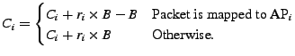
We formalize the scheduling problem as follows. The scheduler is given
a set of accessible APs. It assigns to each AP a value and a cost.
The value of connecting to a particular AP is its contribution to
client throughput. If ![]() is the fraction of time spent at AP
is the fraction of time spent at AP![]() ,
and
,
and ![]() is AP
is AP![]() 's wireless available bandwidth, then the value of
connecting to AP
's wireless available bandwidth, then the value of
connecting to AP![]() is:
is:
The cost of an AP is equal to the time that a client has to spend on
it to collect its value. The cost also involves a setup delay to pick
up in-flight packets and re-tune the card to a new channel. Note that
the setup delay is incurred only when the scheduler spends a non-zero
amount of time at AP![]() . Hence, the cost of AP
. Hence, the cost of AP![]() is:
is:
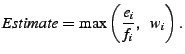
The objective of the scheduler is to maximize client throughput. The
scheduler, however, cannot have too large a duty cycle. If it did,
the delay can hamper the TCP connections, increasing their RTTs,
causing poor throughput and potential time-outs. The objective of the
scheduler is to pick the ![]() 's to maximize the switching value
subject to two constraints: the cost in time must be no more than the
chosen duty cycle,
's to maximize the switching value
subject to two constraints: the cost in time must be no more than the
chosen duty cycle, ![]() , and the fraction of time at an AP has to be
positive and no more than
, and the fraction of time at an AP has to be
positive and no more than
![]() , i.e.,
, i.e.,
How do we solve this optimization? In fact, the optimization problem
in Eqs. 4-6 is similar to the known knapsack
problem [3]. Given a set of items, each with a value and a
weight, we would like to pack a knapsack so as to maximize the total
value subject to a constraint on the total weight. Our items (the
APs) have both fractional weights (costs)
![]() and zero-one
weights
and zero-one
weights
![]() . The knapsack problem is
typically solved using dynamic programming. The formulation of this
dynamic programming solution is well-known and can be used for our
problem [3].
. The knapsack problem is
typically solved using dynamic programming. The formulation of this
dynamic programming solution is well-known and can be used for our
problem [3].
A few points are worth noting.
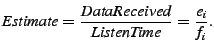
How does a client estimate the uplink wireless available bandwidth? The
client can estimate it by measuring the time between when a packet
reaches the head of the transmit queue and when the packet is acked by
the AP. This is the time taken to deliver one packet, ![]() , given
contention for the medium, autorate, retransmissions, etc. We estimate
the available wireless bandwidth by dividing the packet's size in
bytes,
, given
contention for the medium, autorate, retransmissions, etc. We estimate
the available wireless bandwidth by dividing the packet's size in
bytes, ![]() , by its delivery time
, by its delivery time ![]() . The client takes an
exponentially weighted average over these measurements to smooth out
variability, while adapting to changes in load and link quality.
. The client takes an
exponentially weighted average over these measurements to smooth out
variability, while adapting to changes in load and link quality.
Next, we explain how we measure the delivery time ![]() . Note that
the delivery time of packet
. Note that
the delivery time of packet ![]() is:
is:
Obtaining ![]() , however, is more complex. The driver hands the
packet to the HAL, which queues it for transmission. The driver does
not know when the packet reaches the head of the transmission
queue. Further, we do not have access to the HAL source, so we cannot
modify it to export the necessary information.1 We work around this issue as follows. We make
the driver timestamp packets just before it hands them to the HAL.
Suppose the timestamp of packet
, however, is more complex. The driver hands the
packet to the HAL, which queues it for transmission. The driver does
not know when the packet reaches the head of the transmission
queue. Further, we do not have access to the HAL source, so we cannot
modify it to export the necessary information.1 We work around this issue as follows. We make
the driver timestamp packets just before it hands them to the HAL.
Suppose the timestamp of packet ![]() as it is pushed to the HAL is
as it is pushed to the HAL is
![]() , we can then estimate
, we can then estimate ![]() as follows:
as follows:
Two practical complications exist however. First, the timer in the HAL
has millisecond accuracy. As a result, the estimate of the delivery
time ![]() in Eq. 7 will be equally coarse, and mostly either
0 ms or 1 ms. To deal with this coarse resolution, we need to
aggregate over a large number of measurements. In particular, FatVAP produces a measurement of the wireless available throughput at AP
in Eq. 7 will be equally coarse, and mostly either
0 ms or 1 ms. To deal with this coarse resolution, we need to
aggregate over a large number of measurements. In particular, FatVAP produces a measurement of the wireless available throughput at AP![]() by taking an average over a window of
by taking an average over a window of ![]() seconds (by default
seconds (by default ![]() s),
as follows:
s),
as follows:
A second practical complication occurs because both the driver's timer and the HAL's timer are typically synchronized with the time at the AP. This synchronization happens with every beacon received from the AP. But as FatVAP switches APs, the timers may resynchronize with a different AP. This is fine in general as both timers are always synchronized with respect to the same AP. The problem, however, is that some of the packets in the transmit queue may have old timestamps taken with respect to the previous AP. To deal with this issue, the FatVAP driver remembers the id of the last packet that was pushed into the HAL. When resynchronization occurs (i.e., the beacon is received), it knows that packets with ids smaller than or equal to the last pushed packet have inaccurate timestamps and should not contribute to the average in Eq. 9.
Finally, we note that FatVAP's estimation of available bandwidth is mostly passive and leverages transmitted data packets. FatVAP uses probes only during initialization, because at that point the client has no traffic traversing the AP. FatVAP also occasionally probes the unused APs (i.e., APs not picked by the scheduler) to check that their available bandwidth has not changed.
How do we measure an AP's end-to-end available bandwidth? The naive
approach would count all bytes received from the AP in a certain time
window and divide the count by the window size. The problem, however,
is that no packets might be received either because the host has not
demanded any, or the sending server is idle. To avoid underestimating
the available bandwidth, FatVAP guesses which of the inter-packet
gaps are caused by idleness and removes those gaps. The algorithm is
fairly simple. It ignores packet gaps larger than one second. It also
ignores gaps between small packets, which are mostly AP beacons and
TCP acks, and focuses on the spacing between pairs of large
packets. After ignoring packet pairs that include small packets and
those that are spaced by excessively long intervals, FatVAP computes
an estimate of the end-to-end available bandwidth at AP![]() as:
as:
![\includegraphics[width=2in, clip]{figures/measurement_fallacy.eps}](img65.png)
|
One subtlety remains however.
When a client re-connects to an AP, the AP first drains out all
packets that it buffered when the client was away. These packets go
out at the wireless available bandwidth ![]() . Once the buffer is
drained out, the remaining data arrives at the end-to-end available
bandwidth
. Once the buffer is
drained out, the remaining data arrives at the end-to-end available
bandwidth ![]() . Since the client receives a portion of its data at
the wireless available bandwidth and
. Since the client receives a portion of its data at
the wireless available bandwidth and
![]() , simply counting
how quickly the bytes are received, as in Eq. 10,
over-estimates the end-to-end available bandwidth.
, simply counting
how quickly the bytes are received, as in Eq. 10,
over-estimates the end-to-end available bandwidth.
Fig. 4 plots how the estimate of end-to-end available
bandwidth
![]() relates to the true value
relates to the true value ![]() . There are
two distinct phases. In one phase, the estimate is equal to
. There are
two distinct phases. In one phase, the estimate is equal to ![]() ,
which is shown by the flat part of the solid blue line. This phase
corresponds to connecting to AP
,
which is shown by the flat part of the solid blue line. This phase
corresponds to connecting to AP![]() for less time than needed to
collect all buffered data, i.e.,
for less time than needed to
collect all buffered data, i.e.,
![]() . Since the
buffered data drains at
. Since the
buffered data drains at ![]() , the estimate will be
, the estimate will be
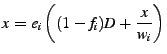
![]() . In the other phase, the estimate is systematically inflated by
. In the other phase, the estimate is systematically inflated by
![]() , as shown by the tilted part of the solid blue line.
This phase corresponds to connecting to AP
, as shown by the tilted part of the solid blue line.
This phase corresponds to connecting to AP![]() for more time than
needed to collect all buffered data, i.e.,
for more time than
needed to collect all buffered data, i.e.,
![]() .
The derivation for this inflation is in
Appendix A. Here, we note the ramifications.
.
The derivation for this inflation is in
Appendix A. Here, we note the ramifications.
Inflated estimates of the end-to-end available bandwidth make the
ideal operating point unstable. A client would ideally operate at the
black dot in Fig. 4, where it connects to AP![]() for
exactly
for
exactly
![]() of its time. But, if the client does
so, the estimate
of its time. But, if the client does
so, the estimate
![]() will be
will be
![]() . In this case, the client cannot figure out
the amount of inflation in
. In this case, the client cannot figure out
the amount of inflation in ![]() and compensate for it because the
true end-to-end available bandwidth can be any value corresponding to
the flat thick blue line in Fig. 4. Even worse, if
the actual end-to-end available bandwidth were to increase, say
because a contending client shuts off, the client cannot observe this
change, because its estimate will still be
and compensate for it because the
true end-to-end available bandwidth can be any value corresponding to
the flat thick blue line in Fig. 4. Even worse, if
the actual end-to-end available bandwidth were to increase, say
because a contending client shuts off, the client cannot observe this
change, because its estimate will still be ![]() .
.
To fix this, FatVAP clients operate at the red dot, i.e., they spend
slightly longer than necessary at each AP in order to obtain an
accurate estimate of the end-to-end bandwidth. Specifically, if
![]() , FatVAP knows that it is operating near or
beyond the black dot and thus slightly increases
, FatVAP knows that it is operating near or
beyond the black dot and thus slightly increases ![]() to go back to
the red dot. The red arrows in the figure show how a FatVAP client
gradually adapts its
to go back to
the red dot. The red arrows in the figure show how a FatVAP client
gradually adapts its ![]() to bring it closer to the desired range. As
long as
to bring it closer to the desired range. As
long as ![]() is larger than the optimal value, we can compensate for
the inflation knowing that
is larger than the optimal value, we can compensate for
the inflation knowing that
![]() , i.e.,
Eq. 10 can be re-written as:
, i.e.,
Eq. 10 can be re-written as:
When splitting traffic, the first question is whether the traffic allocation unit should be a packet, a flow, or a destination? FatVAP allocates traffic to APs on a flow-by-flow basis. A flow is identified by its destination IP address and its ports. FatVAP records the flow-to-AP mapping in a hash-table. When a new flow arrives, FatVAP decides which AP to assign this flow to and records the assignment in the hash table. Subsequent packets in the flow are simply sent through the AP recorded in the hash table.
Our decision to pin flows to APs is driven by practical considerations. First, it is both cumbersome and inefficient to divide traffic at a granularity smaller than a flow. Different APs usually use different DHCP servers and accept traffic only when the client uses the IP address provided by the AP's DHCP server. This means that in the general case, a flow cannot be split across APs. Further, splitting a TCP flow across multiple paths often reorders the flow's packets hurting TCP performance [25]. Second, a host often has many concurrent flows, making it easy to load balance traffic while pinning flows to APs. Even a single application can generate many flows. For example, browsers open parallel connections to quickly fetch the objects in a web page (e.g., images, scripts) [18], and file-sharing applications like BitTorrent open concurrent connections to peers.
But, how do we assign flows to APs to satisfy the ratios in
Eq.12? The direct approach assigns a new flow to the
i![]() AP with a random probability
AP with a random probability ![]() . Random assignment works
when the flows have similar sizes. But flows vary significantly in
their sizes and
rates [15,22,25]. To deal with
this issue, FatVAP maintains per-AP token counters,
. Random assignment works
when the flows have similar sizes. But flows vary significantly in
their sizes and
rates [15,22,25]. To deal with
this issue, FatVAP maintains per-AP token counters, ![]() , that reflect
the deficit of each AP, i.e., how far the number of bytes mapped to an
AP is from its desired allocation. For every packet,
FatVAP increments all counters proportionally to the APs' ratios in
Eq. 12. The counter of the AP that the packet was
sent/received on is decremented by the packet size
, that reflect
the deficit of each AP, i.e., how far the number of bytes mapped to an
AP is from its desired allocation. For every packet,
FatVAP increments all counters proportionally to the APs' ratios in
Eq. 12. The counter of the AP that the packet was
sent/received on is decremented by the packet size ![]() . Hence, every
window of
. Hence, every
window of ![]() seconds (default is
seconds (default is ![]() s) we compute:
s) we compute:
 |
(13) |
To address this issue, FatVAP uses a reverse NAT as a shim between the APs and the kernel, as shown in Fig. 5. Given a single physical wireless card, the FatVAP driver exposes just one interface with a dummy IP address to the kernel. To the rest of the MadWifi driver, however, FatVAP pretends that the single card is multiple interfaces. Each of the interfaces is associated to a different AP, using a different IP address. Transparent to the host kernel, FatVAP resets the addresses in a packet so that the packet can go through its assigned AP.
On the send side, and as shown in Fig. 6, FatVAP
modifies packets just as they enter the driver from the kernel. If
the flow is not already pinned to an AP, FatVAP uses the load
balancing algorithm above to pin this new flow to an AP. FatVAP then
replaces the source IP address in the packet with the IP address of
the interface that is associated with the AP. Of course, this means
that the IP checksum has to be re-done. Rather than recompute the
checksum of the entire packet, FatVAP uses the fact that the checksum
is a linear code over the bytes in the packet. So analogous
to [14], the checksum is recomputed by subtracting some
![]() the dummy IP address
the dummy IP address![]() and adding
and adding
![]() assigned
interface's IP
assigned
interface's IP![]() . Similarly, transport layer checksums, e.g., TCP
and UDP checksums, need to be redone as these protocols use the IP
header in their checksum computation. After this, FatVAP hands over
the packet to standard MadWifi processing, as if this were a packet
the kernel wants to transmit out of the assigned interface.
. Similarly, transport layer checksums, e.g., TCP
and UDP checksums, need to be redone as these protocols use the IP
header in their checksum computation. After this, FatVAP hands over
the packet to standard MadWifi processing, as if this were a packet
the kernel wants to transmit out of the assigned interface.
On the receive side, FatVAP modifies packets after standard MadWifi processing, just before they are handed up to the kernel. If the packet is not a broadcast packet, FatVAP replaces the IP address of the actual interface the packet was received on with the dummy IP of the interface the kernel is expecting the packets on. Checksums are re-done as on the send side, and the packet is handed off to the kernel.
So, how do we leverage this idea for quickly switching APs without losing packets? Two fundamental issues need to be solved. First, when switching APs, what does one do with packets inside the driver destined for the old AP? An AP switching system that sits outside the driver, like MultiNet [13] has no choice but to wait until all packets queued in the driver are drained, which could take a while. Systems that switch infrequently, such as MadWifi that does so to scan in the background, drop all the queued packets. To make AP switching fast and loss-free, FatVAP pushes the switching procedure to the driver, where it maintains multiple transmit queues, one for each interface. Switching APs simply means detaching the old AP's queue and reattaching the new AP's queue. This makes switching a roughly constant time operation and avoids dropping packets. It should be noted that packets are pushed to the transmit queue by the driver and read by the HAL. Thus, FatVAP still needs to wait to resolve the state of the head of the queue. This is, however, a much shorter wait (a few milliseconds) with negligible impact on TCP and the scheduler.
Second, how do we maintain multiple 802.11 state machines simultaneously within a single driver? Connecting with an AP means maintaining an 802.11 state machine. For example, in 802.11, a client transitions from INIT to SCAN to AUTH to ASSOC before reaching RUN, where it can forward data through the AP. It is crucial to handle state transitions correctly because otherwise no communication may be possible. For example, if an association request from one interface to its AP is sent out when another interface is connected to its AP, perhaps on a different channel, the association will fail preventing further communication. To maintain multiple state machines simultaneously, FatVAP adds hooks to MadWifi's 802.11 state-machine implementation. These hooks trap all state transitions in the driver. Only transitions for the interface that is currently connected to its AP can proceed, all other transitions are held pending and handled when the interface is scheduled next. Passive changes to the state of an interface such as receiving packets or updating statistics are allowed at all times.
|
Fig. 7 summarizes the FatVAP drivers' actions when switching from an old interface-AP pair to a new pair.
(a) Cannot Use a Single MAC Address: When two APs are on the same 802.11 channel (operate in the same frequency band), as in Fig. 8a, you cannot connect to both APs with virtual interfaces that have the same MAC address. To see why this is the case, suppose the client uses both AP1 and AP2 that are on the same 802.11 channel. While exchanging packets with AP2, the client claims to AP1 that it has gone into the power-save mode. Unfortunately, AP1 overhears the client talking to AP2 as it is on the same channel, concludes that the client is out of power-save mode, tries to send the client its buffered packets and when un-successful, forcefully deauthenticates the client.
FatVAP confronts MAC address problems with an existing feature in many wireless chipsets that allows a physical card to have multiple MAC addresses [4]. The trick is to change a few of the most significant bits across these addresses so that the hardware can efficiently listen for packets on all addresses. But, of course, the number of such MAC addresses that a card can fake is limited. Since the same MAC address can be reused for APs that are on different channels, FatVAP creates a pool of interfaces, half of which have the primary MAC, and the rest have unique MACs. When FatVAP assigns a MAC address to a virtual interface, it ensures that interfaces connected to APs on the same channel do not share the MAC address.
(b) Light-Weight APs (LWAP): Some vendors allow a physical AP to pretend to be multiple APs with different ESSIDs and different MAC addresses that listen on the same channel, as shown in Fig. 8b. This feature is often used to provide different levels of security (e.g., one light-weight AP uses WEP keys and the other is open) and traffic engineering (e.g., preferentially treat authenticated traffic). For our purpose of aggregating AP bandwidth, switching between light weight APs is useless as the two APs are physically one AP.
FatVAP uses a heuristic to identify light-weight APs. LWAPs that are actually the same physical AP share many bits in their MAC addresses. FatVAP connects to only one AP from any set of APs that have fewer than five bits different in their MAC addresses.
Our results reveal three main findings.
(c) Wireless Clients: We have tested with a few different wireless cards, from the Atheros chipsets in the latest Thinkpads (Atheros AR5006EX) to older Dlink and Netgear cards. Clients are 2GHz x86 machines that run Linux v2.6. In each experiment, we make sure that FatVAP and the compared unmodified driver use similar machines with the same kernel version/revision and the same card.
(d) Traffic Shaping: To emulate an AP backhaul link, we add a traffic shaper behind each of our test-bed APs. This shaper is a Linux box that bridges the APs traffic to the Internet and has two Ethernet cards, one of which is plugged into the lab's (wired) GigE infrastructure, and the other is connected to the AP. The shaper controls the end-to-end bandwidth through a token bucket based rate-filter whose rate determines the capacity of AP's access link. We use the same access capacity for both downlink and uplink.
|
Table 1 shows our microbenchmarks. The table shows that the delay seen by packets on the fast-path (e.g., flow lookup to find which AP the packets need to go to, re-computing checksums) is negligible. Similarly, the overhead of computing and updating the scheduler is minimal. The bulk of the overhead is caused by AP switching. It takes an average of 3 ms to switch from one AP to another. This time includes sending a power save frame, waiting until the HAL has finished sending/receiving the current packet, switching both the transmit and receive queues, switching channel/AP, and sending a management frame to the new AP informing it that the client is back from power save mode. The standard deviation is also about 3 ms, owing to the variable amount of pending interrupts that have to be picked up. Because FatVAP performs AP switching in the driver, its average switching delay is much lower than prior systems (3ms as opposed to 30-600ms). We note that switching cost directly affects the throughput a user can get. A user switching between two APs every 100ms, would only have 40ms of usable time left if each switch takes 30ms, as opposed to 94ms of usable time when each switch takes 3ms and hence can more than double his throughput (94% vs. 40% use).
|
Our experimental setup shown in Fig. 9(a) has
![]() APs. The APs are on different channels and each AP
has a relatively thin access link to the Internet (capacity
APs. The APs are on different channels and each AP
has a relatively thin access link to the Internet (capacity ![]() Mb/s),
which we emulate using the traffic shaper described
in §4.1(c). The wireless bandwidth to the APs is about
Mb/s),
which we emulate using the traffic shaper described
in §4.1(c). The wireless bandwidth to the APs is about
![]() Mb/s. The traffic constitutes of long-lived iperf TCP flows,
and there are as many TCPs as APs, as described
in §4.1(d). Each experiment is first performed by
FatVAP, then repeated with an unmodified driver. We perform 20 runs
and compute the average throughput across them. The question we ask
is: does FatVAP present its client with a fat virtual AP, whose
backhaul bandwidth is the sum of the AP's backhaul bandwidths?
Mb/s. The traffic constitutes of long-lived iperf TCP flows,
and there are as many TCPs as APs, as described
in §4.1(d). Each experiment is first performed by
FatVAP, then repeated with an unmodified driver. We perform 20 runs
and compute the average throughput across them. The question we ask
is: does FatVAP present its client with a fat virtual AP, whose
backhaul bandwidth is the sum of the AP's backhaul bandwidths?
Figs. 9(b) and 9(c) show the aggregate
throughput of the FatVAP client both on the uplink and downlink, as a
function of the number of APs that FatVAP is allowed to access. When
FatVAP is limited to a single AP, the TCP throughput is similar to
running the same experiment with an unmodified client. Both
throughputs are about ![]() Mb/s, slightly less than the access
capacity because of TCP's sawtooth behavior. But as FatVAP is given
access to more APs, its throughput doubles, and triples. At 3 APs,
FatVAP's throughput is
Mb/s, slightly less than the access
capacity because of TCP's sawtooth behavior. But as FatVAP is given
access to more APs, its throughput doubles, and triples. At 3 APs,
FatVAP's throughput is ![]() times larger than the throughput of the
unmodified driver. As the number of APs increases further, we start
hitting the maximum wireless bandwidth, which is about 20-22Mb/s. Note
that FatVAP's throughput stays slightly less than the maximum wireless
bandwidth due to the time lost in switching between APs. FatVAP achieves its maximum throughput when it uses 4 APs. In fact, as a
consequence of switching overhead, FatVAP chooses not to use the fifth
AP even when allowed access to it. Thus, one can conclude that FatVAP effectively aggregates AP backhaul bandwidth up to the limitation
imposed by the maximum wireless bandwidth.
times larger than the throughput of the
unmodified driver. As the number of APs increases further, we start
hitting the maximum wireless bandwidth, which is about 20-22Mb/s. Note
that FatVAP's throughput stays slightly less than the maximum wireless
bandwidth due to the time lost in switching between APs. FatVAP achieves its maximum throughput when it uses 4 APs. In fact, as a
consequence of switching overhead, FatVAP chooses not to use the fifth
AP even when allowed access to it. Thus, one can conclude that FatVAP effectively aggregates AP backhaul bandwidth up to the limitation
imposed by the maximum wireless bandwidth.
|
Fig. 10(b) shows the client throughput, averaged over 2s intervals, as a function of time. The figure shows that if the client uses an unmodified driver connected to AP1, its throughput will change from 15Mb/s to 5Mb/s in accordance with the change in the available bandwidth on that AP. FatVAP, however, achieves a throughput of about 18 Mb/s, and is limited by the sum of the APs' access capacities rather than the access capacity of a single AP. FatVAP also adapts to changes in AP available bandwidth, and maintains its high throughput across such changes.
Fig. 11(b) shows that FatVAP effectively balances the utilization of the APs' access links, whereas the unmodified driver uses only one AP, congesting its access link. Fig. 11(c) shows the corresponding response times. It shows that FatVAP's ability to balance the load across APs directly translates to lower response times for Web requests. While the unmodified driver congests the default APs causing long queues, packet drops, TCP timeouts, and thus long response times, FatVAP balances AP loads to within in a few percent, preventing congestion, and resulting in much shorter response times.
|
Fig. 12(b) plots the throughput of both FatVAP and an
unmodified driver when we impose different time-sharing schedules on
FatVAP. For reference, we also plot a horizontal line at ![]() Mb/s, which
is one half of AP1's access capacity. The figure shows that regardless
of how much time FatVAP connects to AP1, it always stays fair to the
unmodified driver, that is, it leaves the unmodified driver about half
of AP1's capacity, and sometimes more. FatVAP achieves the best
throughput when it spends about 55-70% of its time on AP1. Its
throughput peaks when it spends about 64% of its time on AP1, which
is, in fact, the solution computed by our scheduler
in §3.1 for the above bandwidth values. This shows
that our AP scheduler is effective in maximizing client throughput.
Mb/s, which
is one half of AP1's access capacity. The figure shows that regardless
of how much time FatVAP connects to AP1, it always stays fair to the
unmodified driver, that is, it leaves the unmodified driver about half
of AP1's capacity, and sometimes more. FatVAP achieves the best
throughput when it spends about 55-70% of its time on AP1. Its
throughput peaks when it spends about 64% of its time on AP1, which
is, in fact, the solution computed by our scheduler
in §3.1 for the above bandwidth values. This shows
that our AP scheduler is effective in maximizing client throughput.
|
Here, we look at ![]() clients that compete for two APs, where AP1 has
2Mb/s of available bandwidth and AP2 has 12 Mb/s, as shown in
Fig. 13(a). The traffic load consists of long-lived
iperf TCP flows, as described
in §4.1(d). Fig. 13(b) plots the average
throughput of clients with and without FatVAP. With an unmodified
driver, clients C1 and C2 associate with AP1, thereby achieving a
throughput of less than 1Mb/s. The remaining clients associate with
AP2 for roughly 4Mb/s throughput for each. However, FatVAP's load
balancing and fine-grained scheduling allow all five clients to fairly
share the aggregate bandwidth of 14 Mb/s, obtaining a throughput of
roughly 2.8 Mb/s each, as shown by the dark bars in
Fig. 13(b).
clients that compete for two APs, where AP1 has
2Mb/s of available bandwidth and AP2 has 12 Mb/s, as shown in
Fig. 13(a). The traffic load consists of long-lived
iperf TCP flows, as described
in §4.1(d). Fig. 13(b) plots the average
throughput of clients with and without FatVAP. With an unmodified
driver, clients C1 and C2 associate with AP1, thereby achieving a
throughput of less than 1Mb/s. The remaining clients associate with
AP2 for roughly 4Mb/s throughput for each. However, FatVAP's load
balancing and fine-grained scheduling allow all five clients to fairly
share the aggregate bandwidth of 14 Mb/s, obtaining a throughput of
roughly 2.8 Mb/s each, as shown by the dark bars in
Fig. 13(b).
|
Fig. 15(a) plots the CDF of throughput taken over all the
web requests in all three locations. The figure shows that FatVAP increases the median throughput in these residential deployments by
![]() x. Fig. 15(b) plots the CDF of the response time
taken over all requests. The figure shows that FatVAP reduces the
median response time by
x. Fig. 15(b) plots the CDF of the response time
taken over all requests. The figure shows that FatVAP reduces the
median response time by ![]() x. Note that though all these locations
have only two APs, Web performance more than doubled. This is due to
FatVAP's ability to balance the load across APs. Specifically, most
Web flows are short lived and have relatively small TCP congestion
windows. Without load balancing, the bottleneck drops a large number
of packets, causing these flows to time out, which results in worse
throughputs and response times. In short, our results show that
FatVAP brings immediate benefit in today's deployments, improving both
client's throughput and response time.
x. Note that though all these locations
have only two APs, Web performance more than doubled. This is due to
FatVAP's ability to balance the load across APs. Specifically, most
Web flows are short lived and have relatively small TCP congestion
windows. Without load balancing, the bottleneck drops a large number
of packets, causing these flows to time out, which results in worse
throughputs and response times. In short, our results show that
FatVAP brings immediate benefit in today's deployments, improving both
client's throughput and response time.
![\includegraphics[width=2.8in, clip]{figures/hotspots_3.eps}](img121.png)
|
The closest to our work is the MultiNet project [13], which was later named VirtualWiFi [6]. MultiNet abstracts a single WLAN card to appear as multiple virtual WLAN cards to the user. The user can then configure each virtual card to connect to a different wireless network. MultiNet applies this idea to extend the reach of APs to far-away clients and to debug poor connectivity. We build on this vision of MultiNet but differ in design and applicability. First, MultiNet provides switching capabilities but says nothing about which APs a client should toggle and how long it should remain connected to an AP to maximize its throughput. In contrast, FatVAP schedules AP switching to maximize throughput and balance load. Second, FatVAP can switch APs at a fine time scale and without dropping packets; this makes it the only system that maintains concurrent TCP connections on multiple APs.
(b) AP Selection: Current drivers select an AP based on signal strength. Prior research has proposed picking an AP based on load [20], potential bandwidth [28], and a combination of metrics [21]. FatVAP fundamentally differs from these techniques in that it does not pick a single AP, but rather multiplexes the various APs in a manner that maximizes client throughput.
(a) Multiple WiFi Cards: While FatVAP benefits from having multiple WiFi cards on the client's machine, it does not rely on their existence. We made this design decision for various reasons. First most wireless equipments naturally come with one card and some small handheld devices cannot support multiple cards. Second, without FatVAP the number of cards equals the number of APs that one can connect with, which limits such a solution to a couple of APs. Third, cards that are placed very close to each other may interfere; WiFi channels overlap in their frequency masks [16] and could leak power to each other's bands particularly if the antennas are placed very close. Forth, even with multiple cards, the client still needs to pick which APs to connect to and route traffic over these APs as to balance the load. FatVAP does not constrain the client to having multiple cards. If the client however happens to have multiple cards, FatVAP would allow the user to exploit this capability to expand the number of APs that it switches between and hence improve the overall throughput.
(b) Channel Bonding and Wider Bands: Advances like channel bonding (802.11n) and wider bands (40MHz wide channels) increase wireless link capacity to hundreds of Mb/s. Such schemes widen the gap between the capacity of the wireless link and the AP's backhaul link, making FatVAP more useful. In such settings, FatVAP lets one wireless card collect bandwidth from tens of APs.
(c) WEP and Splash Screens: We are in the process of adding WEP
and splash-screen login support to our FatVAP prototype. Supporting
WEP keys is relatively easy, the user needs to provide a WEP key for
every secure AP that he wants to access. FatVAP reads a pool of known
![]() WEP key, ESSID
WEP key, ESSID![]() tuples and uses the right key to talk to each
protected AP. Supporting splash screen logins used by some commercial
hot-spots, is a bit more complex. One would need to pin all traffic to
an AP for the duration of authentication, after which FatVAP can
distribute traffic as usual.
tuples and uses the right key to talk to each
protected AP. Supporting splash screen logins used by some commercial
hot-spots, is a bit more complex. One would need to pin all traffic to
an AP for the duration of authentication, after which FatVAP can
distribute traffic as usual.
 |
(18) |
This document was generated using the LaTeX2HTML translator Version 2002-2-1 (1.71)
Copyright © 1993, 1994, 1995, 1996,
Nikos Drakos,
Computer Based Learning Unit, University of Leeds.
Copyright © 1997, 1998, 1999,
Ross Moore,
Mathematics Department, Macquarie University, Sydney.
The command line arguments were:
latex2html -split 0 -no_navigation -white -show_section_numbers paper_htmlsource.tex
The translation was initiated by Srikanth Kandula on 2008-02-24
![\includegraphics[width=3.1in, clip]{figures/example-1-1.eps}](img18.png)


![\includegraphics[width=2.5in, clip]{figures/arch-3.eps}](img77.png)
![\includegraphics[width=1.38in, clip]{figures/send-side.eps}](img78.png)
![\includegraphics[width=1.15in, clip]{figures/receive-side.eps}](img79.png)

![\includegraphics[width=3.2in, clip]{figures/switching.eps}](img93.png)
![\includegraphics[width=1.9in, clip]{figures/pract1_same_chan.eps}](img94.png)
![\includegraphics[width=1.5in, clip]{figures/pract3_same_ap.eps}](img95.png)
![\includegraphics[height=1.1in, clip]{figures/topo-agg-1.eps}](img98.png)
![\includegraphics[width=2.6in, clip]{figures/upper-rx.eps}](img99.png)
![\includegraphics[width=2.6in, clip]{figures/upper-tx.eps}](img100.png)
![\includegraphics[height=1.3in, clip]{figures/topo-dyn.eps}](img101.png)
![\includegraphics[width=3in, clip]{figures/aggr-rx.eps}](img102.png)
![\includegraphics[height=1.3in, clip]{figures/topo-balance.eps}](img107.png)
![\includegraphics[width=2.7in, clip]{figures/load-balance.eps}](img108.png)
![\includegraphics[width=2.5in, clip]{figures/load-rpt.eps}](img109.png)
![\includegraphics[height=1.3in, clip]{figures/topo-compete-fair.eps}](img110.png)
![\includegraphics[width=3in, clip]{figures/fair-rx.eps}](img111.png)
![\includegraphics[height=1.3in, clip]{figures/topo-contend-2.eps}](img116.png)
![\includegraphics[width=3in, clip]{figures/multic-rx.eps}](img117.png)
![\includegraphics[width=2.4in, clip]{figures/graphic.eps}](img118.png)
![\includegraphics[width=2.8in, clip]{figures/home-tput.eps}](img119.png)
![\includegraphics[width=2.8in, clip]{figures/home-rpt.eps}](img120.png)