
[
]
San Fermín is a system for aggregating large amounts of data from the nodes of large-scale distributed systems. Each San Fermín node individually computes the aggregated result by swapping data with other nodes to dynamically create its own binomial tree. Nodes that fall behind abort their trees, thereby reducing overhead. Having each node create its own binomial tree makes San Fermín highly resilient to failures and ensures that the internal nodes of the tree have high capacity, thereby reducing completion time.
Compared to existing solutions, San Fermín handles large aggregations better, has higher completeness when nodes fail, computes the result faster, and has better scalability. We analyze the completion time, completeness, and overhead of San Fermín versus existing solutions using analytical models, simulation, and experimentation with a prototype built on peer-to-peer system deployed on PlanetLab. Our evaluation shows that San Fermín is scalable both in the number of nodes and in the aggregated data size. San Fermín aggregates large amounts of data significantly faster than existing solutions: compared to SDIMS, an existing aggregation system, San Fermín computes a 1MB result from 100 PlanetLab nodes in 61-76% of the time and from 2-6 times as many nodes. Even if 10% of the nodes fail during aggregation, San Fermín still includes the data from 97% of the nodes in the result and does so faster than the underlying peer-to-peer system recovers from failures.
San Fermín aggregates large amounts of data from distributed nodes quickly and accurately. As distributed systems become more prevalent this is an increasingly important operation: for example, CERT logs about 1/4 TB of data daily on approximately 100 nodes distributed throughout the Internet [9]. Analysts use these logs to detect anomalous behavior that signals worms and other attacks, and must do so quickly to minimize damage. An example query might request the number of flows to and from each TCP/UDP port (to detect an anomalous distribution of traffic indicating an attack). In this example there are many flow counters per node and the requester is interested in the sum of each counter across all nodes. It is important that the data be aggregated quickly, as time is of the essence when responding to attacks, and accurately, as the aggregated result should include data from as many nodes as possible and the data from each node exactly once. The more accurate the result, the more useful it is.
In San Fermín the properties of current networks are leveraged to build an efficient content aggregation network for large data sizes. Since core bandwidth is typically not the bottleneck [12], San Fermín allows disjoint pairs of nodes to communicate simultaneously, as they will likely not compete for bandwidth. A San Fermín node also sends and receives data simultaneously, making efficient use of full-duplex links. The result is that San Fermín aggregates large data sets significantly faster than existing solutions, on average returning a 1 MB aggregation from 100 PlanetLab nodes in 61-76% the time and from approximately 2-6 times as many nodes as SDIMS, an existing aggregation system. San Fermín is highly failure resistant and with 10% node failures during aggregation still includes the data from over 97% of the nodes in the result -- and in most cases does so faster than the underlying peer-to-peer system recovers from failures.
San Fermín uses a binomial swap forest to perform the aggregation, which is well-suited to tolerate failures and take advantage of the characteristics of the Internet. In a binomial swap forest each node creates its own binomial tree by repeatedly swapping aggregate data with other nodes. This makes San Fermín highly resilient to failures because a particular node's data is aggregated by an exponentially increasing number of nodes as the aggregation progresses. Similarly, the number of nodes included in a particular node's aggregate data also increases exponentially as the aggregation progresses. Each node creates its own binomial swap tree; as long as at least one node remains alive San Fermín will produce a (possibly incomplete) aggregation result.
Having each node create its own binomial swap tree is highly fault-tolerant and fast, but it can lead to excessive overhead. San Fermín reduces overhead by pruning small trees that fall behind larger trees during the aggregation, as the small trees are unlikely to compute the result first and therefore increase overhead without improving speed or accuracy. When a tree falls behind San Fermín prunes it -- the name San Fermín is derived from this behavior, after the festival with the running of the bulls in Pampalona.
In addition to CERT, San Fermín also benefits other applications that aggregate large amounts of data from many nodes:
Software Debugging Recent work on software debugging [19] leverages execution counts for individual instructions. This work shows that the total of all the instruction execution counts across multiple nodes helps the developer quickly identify bugs.
System Monitoring Administrators of distributed systems must process the logs of thousands of nodes around the world to troubleshoot difficulties, track intrusions, or monitor performance.
Distributed Databases A common query in relational databases is GROUP BY [25]. This query combines table rows containing the same attribute value using an aggregate operator (such as SUM). The query result contains one table row per unique attribute value. In distributed databases different nodes may store rows with the same attribute value. The values at these rows must be combined and returned to the requester.
These applications are similar because they aggregate large amounts of data from many nodes. For example, for the CERT example, finding the distribution of ports on UDP and TCP flows seen in the last hour takes 512 KB (assuming 4 byte counters). In the software debugging application, tracking a small application like bc requires 40KB of counters. Larger applications may require more than 1MB of counters. The target environments may contain hundreds or thousands of nodes, forcing the aggregation to tolerate failures.
The aggregation function has similar characteristics for these applications as well. The aggregation functions are commutative and associative but may be sensitive to duplication. Typically, the aggregate data from multiple nodes is approximately the same size as any individual node's data.
The aggregation functions may also be sensitive to partial data in the result. If, for example, the data from a node is split and aggregated separately using different trees, the root may receive only some of the node's data. For applications that want distributions of data (such as the target applications) it may be important to either have all of a node's data or none of it.
In some cases it may be possible to compress aggregate data before transmission to reduce space. Such techniques are complimentary to this work. Some environments may require administrative isolation. This work assumes that the aggregation occurs in a single administrative domain with cooperative nodes.
[width=38mm]binomialswap.eps
|
A binomial swap forest is a novel technique for aggregating data in which each node
individually computes the aggregate result by repeatedly swapping (exchanging) aggregate data
with other nodes. Two nodes swap data by sending each other the data they have aggregated so far,
allowing each to compute the aggregation of both nodes' data.
The swaps are organized so that a node only swaps with one other node at a time, and
each swap roughly doubles the number of nodes whose data is included in a
node's aggregate data, so that the nodes will compute
the aggregate result in
roughly ![]() swaps.
If the nodes of the aggregation are represented as nodes in a graph,
and swaps as edges in the graph, the
sequence of swaps performed by a particular node form a binomial tree with
that node at the root.
As a reminder, in a binomial tree with
swaps.
If the nodes of the aggregation are represented as nodes in a graph,
and swaps as edges in the graph, the
sequence of swaps performed by a particular node form a binomial tree with
that node at the root.
As a reminder, in a binomial tree with ![]() nodes the children of the root
are themselves binomial trees with
nodes the children of the root
are themselves binomial trees with ![]() ,
, ![]() ...,
..., ![]() , and
, and ![]() nodes
(Figure 1).
As the figure illustrates,
a binomial tree with
nodes
(Figure 1).
As the figure illustrates,
a binomial tree with ![]() nodes can be made from two binomial trees with
nodes can be made from two binomial trees with ![]() nodes
by making
one tree a child of the other tree's root .
The collection of binomial swap trees constructed by the nodes during a single aggregation is a
binomial swap forest.
nodes
by making
one tree a child of the other tree's root .
The collection of binomial swap trees constructed by the nodes during a single aggregation is a
binomial swap forest.
[width=40mm]abcd.eps
|
For example, consider data aggregation from four nodes: A, B, C, and D (Figure 2). Each node initially finds a partner with whom to swap data. Suppose A swaps with B and C swaps with D, so that afterwards A and B have the aggregate data AB, while C and D have the aggregate data CD. To complete the aggregation each node must swap data with a node from the other pair. If A swaps with C and B swaps with D, then every node will have the aggregate data ABCD .
The swaps
must be carefully organized
so that the series of swaps by a node produces the correct aggregated result.
Consider aggregating data from ![]() nodes each with a
unique ID in the range
nodes each with a
unique ID in the range ![]() (we will later relax these constraints).
Since each swap doubles the amount of aggregate data a node has, just prior to the last swap
a node must have the data from half of the nodes in the system, and must swap with a node
that has the data from the other half of the nodes.
This can be achieved by swapping based on node IDs; specifically, if the node ID for a node
(we will later relax these constraints).
Since each swap doubles the amount of aggregate data a node has, just prior to the last swap
a node must have the data from half of the nodes in the system, and must swap with a node
that has the data from the other half of the nodes.
This can be achieved by swapping based on node IDs; specifically, if the node ID for a node ![]() starts with
a 0 then node
starts with
a 0 then node ![]() should aggregate data from all nodes that start with a 0 prior to the
last swap, then swap with a node
should aggregate data from all nodes that start with a 0 prior to the
last swap, then swap with a node ![]() whose node ID starts with 1 that has aggregated
data from all nodes that start with a 1.
Note that it doesn't matter
which node
whose node ID starts with 1 that has aggregated
data from all nodes that start with a 1.
Note that it doesn't matter
which node ![]() node
node ![]() swaps with as long as its node ID starts with a 1 and it has successfully
aggregated data from its half of the node ID space.
Also note that node
swaps with as long as its node ID starts with a 1 and it has successfully
aggregated data from its half of the node ID space.
Also note that node ![]() should swap with exactly one node from the other half of the address space,
otherwise the result may contain duplicate data.
Recursing on this idea, assuming that node
should swap with exactly one node from the other half of the address space,
otherwise the result may contain duplicate data.
Recursing on this idea, assuming that node ![]() starts with 00 then in the penultimate swap it must swap with
a node whose node ID starts with 01 thus aggregating data from all
nodes that start with 0. Similarly,
in the very first swap node
starts with 00 then in the penultimate swap it must swap with
a node whose node ID starts with 01 thus aggregating data from all
nodes that start with 0. Similarly,
in the very first swap node ![]() swaps with the node whose node ID differs in only the
least-significant bit.
This is the general idea behind
using a binomial swap forest to aggregate data -- each node starts
by swapping data with the node
whose node ID differs in only the least-significant bit
and works its way through the node ID space until
it swaps with a node whose node ID differs in the most-significant bit.
swaps with the node whose node ID differs in only the
least-significant bit.
This is the general idea behind
using a binomial swap forest to aggregate data -- each node starts
by swapping data with the node
whose node ID differs in only the least-significant bit
and works its way through the node ID space until
it swaps with a node whose node ID differs in the most-significant bit.
 |
[width=70mm]binomialforestsquashed.eps
|
Before describing this process in more detail it is useful to define the longest common prefix,
![]() of two nodes, which is the number of high-order bits the two node IDs have in common.
We will use the notation
of two nodes, which is the number of high-order bits the two node IDs have in common.
We will use the notation
![]() to mean that the
to mean that the
![]() of nodes
of nodes ![]() and
and ![]() is
is ![]() bits long.
With respect to a particular node
bits long.
With respect to a particular node ![]() , we use the notation
, we use the notation
![]() to indicate the set of nodes
whose longest common prefix with node
to indicate the set of nodes
whose longest common prefix with node ![]() is
is ![]() bits long.
We shorten this to
bits long.
We shorten this to
![]() when it is clear which node
when it is clear which node ![]() is being referred to.
is being referred to.
Using this notation, to aggregate data using a binomial swap tree in a system
with ![]() nodes a node
nodes a node ![]() must first swap data with a node in
must first swap data with a node in
![]() (there is only 1 node
in this set), then swap data with a node in
(there is only 1 node
in this set), then swap data with a node in
![]() , etc., until eventually
swapping data with a node in
, etc., until eventually
swapping data with a node in
![]() (there are
(there are ![]() nodes in this set).
Again, node
nodes in this set).
Again, node ![]() swaps with only one node in
swaps with only one node in
![]() to prevent duplication in the result.
Each set
to prevent duplication in the result.
Each set
![]() has
has ![]() nodes,
and
node
nodes,
and
node ![]() will perform
will perform ![]() swaps. Duplication cannot happen because
when node
swaps. Duplication cannot happen because
when node ![]() swaps data with node
swaps data with node ![]() from set
from set
![]() , node
, node ![]() receives the data
from nodes whose longest common prefix with node
receives the data
from nodes whose longest common prefix with node ![]() is exactly
is exactly ![]() bits long.
To see why this is true, consider that
bits long.
To see why this is true, consider that ![]() has data from all nodes
whose longest common prefix with
has data from all nodes
whose longest common prefix with ![]() is at least
is at least ![]() bits. This
means that the first
bits. This
means that the first ![]() bits of these nodes are the same as
bits of these nodes are the same as ![]() and since
and since ![]() differs with
differs with ![]() in the
in the ![]() th bit,
th bit, ![]() must differ with these nodes in the
must differ with these nodes in the
![]() th bit.
th bit.
The discussion so far assumes that the number of nodes in the system is a power of 2,
that node IDs are in the range ![]() , that
each node knows how to contact every other node in the system directly, and that
nodes do not fail. It also ignores the overhead of having each node construct
its own binomial swap tree when only a single tree is necessary to compute the aggregated
result. We can relax the first of these restrictions to allow the number of nodes to not
be a power of 2, but it introduces several complications. First,
the resulting binomial trees will not be complete, although they will produce the
correct aggregate result.
Consider data aggregation in
a system with only
nodes A, B, and C. Suppose A initially swaps with B. C
must wait for A and B to finish swapping before it can swap with one of them.
Suppose C subsequently swaps with A, so that both A and C have the aggregate data ABC,
while node B only has AB. A and C
successfully computed the result although the binomial trees they constructed are not
complete. B was unable to construct a tree containing all the nodes.
, that
each node knows how to contact every other node in the system directly, and that
nodes do not fail. It also ignores the overhead of having each node construct
its own binomial swap tree when only a single tree is necessary to compute the aggregated
result. We can relax the first of these restrictions to allow the number of nodes to not
be a power of 2, but it introduces several complications. First,
the resulting binomial trees will not be complete, although they will produce the
correct aggregate result.
Consider data aggregation in
a system with only
nodes A, B, and C. Suppose A initially swaps with B. C
must wait for A and B to finish swapping before it can swap with one of them.
Suppose C subsequently swaps with A, so that both A and C have the aggregate data ABC,
while node B only has AB. A and C
successfully computed the result although the binomial trees they constructed are not
complete. B was unable to construct a tree containing all the nodes.
Second,
some nodes may not be able to find partners with whom to swap, as is the case with
node B in the previous example.
More generally,
consider a collection of nodes whose longest common prefix
![]() is
is ![]() bits long.
To aggregate the data for that prefix the subset of nodes whose
bits long.
To aggregate the data for that prefix the subset of nodes whose
![]() ends with a 0
must swap data with the subset whose
ends with a 0
must swap data with the subset whose
![]() ends with a 1. If these subsets are not
of equal size, then some nodes will be unable to find a partner.
Only if
ends with a 1. If these subsets are not
of equal size, then some nodes will be unable to find a partner.
Only if ![]() is a power of 2 can the two subsets have equal numbers of nodes,
otherwise some nodes will be unable to find a partner and must abort their aggregations.
is a power of 2 can the two subsets have equal numbers of nodes,
otherwise some nodes will be unable to find a partner and must abort their aggregations.
Third, if the number of nodes is not a power of 2 then some node IDs will
not be assigned to nodes. This can result in no nodes having a particular prefix,
so that when other nodes try to swap with nodes having that prefix they cannot
find a partner with whom to swap. Instead of aborting those nodes should instead
simply skip the prefix as it is empty. This is most likely to occur when the nodes
initially start the aggregation process, as for any node ![]()
![]() corresponds
to exactly one node ID, which may not be assigned to a node. Therefore, instead of
starting the aggregation with
corresponds
to exactly one node ID, which may not be assigned to a node. Therefore, instead of
starting the aggregation with
![]() node
node ![]() should instead
initially swap with a node in
should instead
initially swap with a node in
![]() where
where ![]() is the longest prefix
length for which
is the longest prefix
length for which
![]() is not empty.
is not empty.
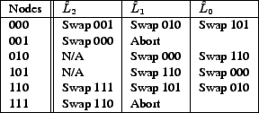
As an example of aggregating data when ![]() is not a power of 2, suppose
that there are 6
nodes: 000, 001, 010, 101, 110, and 111 (Figures 3 and 4).
Each node
is not a power of 2, suppose
that there are 6
nodes: 000, 001, 010, 101, 110, and 111 (Figures 3 and 4).
Each node ![]() swaps data with a node in each
swaps data with a node in each
![]() starting with
starting with
![]() and ending with
and ending with
![]() .
There are many valid binomial swap forests that could be constructed by these nodes
aggregating data; in this example 000 first swaps with 001 and 110 swaps with
111.
.
There are many valid binomial swap forests that could be constructed by these nodes
aggregating data; in this example 000 first swaps with 001 and 110 swaps with
111.
![]() is empty for 010 and 101, so they swap with nodes in
is empty for 010 and 101, so they swap with nodes in
![]() :
000 swaps with 010 and 101 swaps with 111. 001 and 110 cannot find a node
in
:
000 swaps with 010 and 101 swaps with 111. 001 and 110 cannot find a node
in
![]() with whom to swap (since 010 swapped with 000 and 101 swapped with
with 111) and they stop aggregating data. In the final step the remaining nodes swap
with a node in
with whom to swap (since 010 swapped with 000 and 101 swapped with
with 111) and they stop aggregating data. In the final step the remaining nodes swap
with a node in
![]() : 000 swaps with 101 and 010 swaps with 111.
: 000 swaps with 101 and 010 swaps with 111.
The swap operations in a binomial swap forest are
only partially ordered - the only constraints are that nodes must
swap with a node in each
![]() in order starting with
in order starting with
![]() and ending with
and ending with
![]() .
It is possible that in
Figure 3 that nodes 000 and 010 will finish swapping
before 111 and 110 finish swapping. This means that the only synchronization
between nodes is when they swap data (there is no global synchronization between nodes).
.
It is possible that in
Figure 3 that nodes 000 and 010 will finish swapping
before 111 and 110 finish swapping. This means that the only synchronization
between nodes is when they swap data (there is no global synchronization between nodes).
San Fermín makes use of an underlying peer-to-peer communication system to handle both gaps in the node ID space and nodes that are not able to communicate directly. It uses time-outs to deal with node failures, and employs a pruning algorithm to reduce overhead by eliminating unprofitable trees. Section 4 these aspects of San Fermín in more detail.
Several techniques have been proposed for content aggregation. The most straightforward is to have a single node retrieve all data and then aggregate. Some techniques like SDIMS [31] build a tree with high-degree nodes that are likely to have simultaneous connections. To provide resilience against failures, data is retransmitted when nodes fail. Seaweed [22] also has high-degree nodes with a similar structure to SDIMS, but uses a supernode approach in which the data on internal nodes are replicated to tolerate failures.
Analytic models of these techniques enable comparison of their
general characteristics.
The models assume that any node that fails
during the aggregation does not recover, and any node that comes online
during the aggregation does not join it. The probability of a given
node failing in the next second is ![]() .
Node failures are assumed to be independent.
A node that fails while sending data causes the partial data to be
discarded. Inter-node latencies and bandwidths are a uniform
.
Node failures are assumed to be independent.
A node that fails while sending data causes the partial data to be
discarded. Inter-node latencies and bandwidths are a uniform ![]() and
and ![]() ,
respectively. The bandwidth
,
respectively. The bandwidth ![]() is per-node,
which is consistent with the
bandwidth bottleneck existing at the edges of the network
and not in the middle. Each node contributes data of size
is per-node,
which is consistent with the
bandwidth bottleneck existing at the edges of the network
and not in the middle. Each node contributes data of size ![]() and
the aggregation function produces aggregate data of size
and
the aggregation function produces aggregate data of size ![]() .
Per-packet, peer-to-peer, and connection establishment costs are ignored for
all techniques.
.
Per-packet, peer-to-peer, and connection establishment costs are ignored for
all techniques.
Other parameters such as the amount of data aggregated, speed and capacity of the links, etc. are derived from real-world measurements (Table 1). The bandwidth measurements were gathered by transferring a 1MB file to all PlanetLab nodes from several well-connected nodes. The average bandwidth was within 100 Kbps for all runs, independent of the choice of source node. This means that well-connected nodes have roughly the same bandwidth to other nodes regardless of network location. The average of all runs is used in Table 1.
|
For each technique its completion time, completeness (number of nodes whose data is included in the aggregate result), and overhead are analyzed. Rather than isolating all of the parameters for each technique, the data size and number of nodes are varied to show their effect.
The analysis of San Fermín assumes a complete binomial
swap forest. Since it takes ![]() time to do a swap, the
completion time is
time to do a swap, the
completion time is
![]() .
Figures 5a and 6a show that using a
binomial swap forest is effective at rapidly aggregating data. For example,
using a binomial swap forest takes less than 1/3 the time of other techniques
when more than 128 KB of data per node is aggregated.
.
Figures 5a and 6a show that using a
binomial swap forest is effective at rapidly aggregating data. For example,
using a binomial swap forest takes less than 1/3 the time of other techniques
when more than 128 KB of data per node is aggregated.
After a node swaps with ![]() other nodes
in a binomial swap forest its data will
appear in
other nodes
in a binomial swap forest its data will
appear in ![]() binomial trees, so that
binomial trees, so that ![]() nodes must fail for the
original node's data to be lost.
The probability of single node failing by time
nodes must fail for the
original node's data to be lost.
The probability of single node failing by time ![]() is
is
![]() , and the probability of
, and the probability of ![]() nodes failing by
time
nodes failing by
time ![]() is
is ![]() . This leads to a completeness of
. This leads to a completeness of
![]() . As Figures 5b and
6b show, a binomial swap forest has
high completeness in the face of failures. For example,
when aggregating more than 64KB of data, a binomial swap
forest loses data from an order of magnitude fewer nodes than the
other techniques.
. As Figures 5b and
6b show, a binomial swap forest has
high completeness in the face of failures. For example,
when aggregating more than 64KB of data, a binomial swap
forest loses data from an order of magnitude fewer nodes than the
other techniques.
Building a binomial swap forest involves each node swapping data with
![]() other nodes. Assuming that failures do not impact overhead,
the overhead is
other nodes. Assuming that failures do not impact overhead,
the overhead is ![]() . As
Figures 5c and 6c show, the
overhead of a binomial swap forest is very high (Section 4
explains how San Fermín reduces this overhead by pruning trees).
Using a binomial swap
forest to aggregate 1MB of data requires about 20 times more overhead than
balanced trees and about 5 times more than supernodes.
. As
Figures 5c and 6c show, the
overhead of a binomial swap forest is very high (Section 4
explains how San Fermín reduces this overhead by pruning trees).
Using a binomial swap
forest to aggregate 1MB of data requires about 20 times more overhead than
balanced trees and about 5 times more than supernodes.
Intuitively, a binomial swap forest works well for two reasons. First, bandwidth dominates when aggregating large amounts of data. Other techniques build trees with higher fan-in so that nodes contend for bandwidth, while a binomial swap forest has no contention since swaps are done with only one node at a time. Second, data is replicated widely so that failures are less likely to reduce completeness. Nodes swap repeatedly, so that an exponential number of nodes need to fail for the data to be lost.
[Completion Time vs. Data Size. ][width=39mm,angle=270]model/ts.out.ps
[Completeness vs. Data Size][width=39mm,angle=270]model/cs.out.ps
[Overhead vs. Data Size][width=39mm,angle=270]model/os.out.ps |
[Completion Time vs. Nodes][width=39mm,angle=270]model/tn.out.ps
[Completeness vs. Nodes][width=39mm,angle=270]model/cn.out.ps
[Overhead vs. Nodes][width=39mm,angle=270]model/on.out.ps |
In the centralized model, a central node contacts every node, retrieves
their data directly, and computes the aggregated result.
The central node can eliminate almost all latency costs by
pipelining the retrievals,
resulting in a completion time of
![]() . This is much higher than the other techniques
shown in Figure 5a because the time is linear in the
number of nodes and the other techniques are logarithmic. As a result,
to aggregate 1MB of data using the centralized technique takes 26 days
as compared to about 2 minutes with a binomial swap forest.
. This is much higher than the other techniques
shown in Figure 5a because the time is linear in the
number of nodes and the other techniques are logarithmic. As a result,
to aggregate 1MB of data using the centralized technique takes 26 days
as compared to about 2 minutes with a binomial swap forest.
The completeness is the number of nodes
that did not fail prior to the central node retrieving their data.
The probability that a node is alive after ![]() seconds
is
seconds
is ![]() , so the expected completeness is
, so the expected completeness is
![]() .
As can be seen in Figures 5b and
6b the centralized model has very poor results,
despite assuming that the central node does not fail.
The poor results are because many nodes fail before they are contacted
by the central node.
.
As can be seen in Figures 5b and
6b the centralized model has very poor results,
despite assuming that the central node does not fail.
The poor results are because many nodes fail before they are contacted
by the central node.
The overhead is the number of nodes that were alive when contacted multiplied
by the data size:
![]() . A comparison is shown in
Figures 5c and 6c.
These results seem fantastic for large data sizes and numbers of nodes when
compared to other algorithms, however what is really happening is that
many nodes fail before their data is retrieved, reducing overhead but
also reducing completeness.
. A comparison is shown in
Figures 5c and 6c.
These results seem fantastic for large data sizes and numbers of nodes when
compared to other algorithms, however what is really happening is that
many nodes fail before their data is retrieved, reducing overhead but
also reducing completeness.
Aggregation is often performed using trees whose internal nodes have
similar degree ![]() and whose leaf nodes have similar depth.
An internal node waits for data from all of its children
before computing the aggregated data and sending the aggregate result to its
parent.
In practice, one of the
child nodes is also the parent node so only
and whose leaf nodes have similar depth.
An internal node waits for data from all of its children
before computing the aggregated data and sending the aggregate result to its
parent.
In practice, one of the
child nodes is also the parent node so only ![]() children send data
to the parent.
The model assumes that trees are balanced and complete with degree
children send data
to the parent.
The model assumes that trees are balanced and complete with degree ![]() .
If the effects of failures on completion time are ignored, the completion
time is
.
If the effects of failures on completion time are ignored, the completion
time is
![]() . As
Figure 5a shows, this algorithm is quite fast when the
data size is small and hence latency dominates.
However, the performance quickly degrades when the
data size increases. Aggregating 1MB of data using a balanced tree
is about 4 times slower than using a binomial swap forest.
. As
Figure 5a shows, this algorithm is quite fast when the
data size is small and hence latency dominates.
However, the performance quickly degrades when the
data size increases. Aggregating 1MB of data using a balanced tree
is about 4 times slower than using a binomial swap forest.
A node that fails before sending to its parent will be missing from the result.
It is also possible that both the child and parent fail after the child has
sent the data, also causing the child to be missing.
The completeness model captures these node failures.
However, the model does
not consider a cascade effect. This occurs when a parent has failed and
another node is recovering the data from the children
when a child fails. The node that recovers and
takes the role of the child would need to recover data from the child's
children. This is failure handling of a child within failure handling of
the parent (a cascade effect) and is not captured in the model.
In the balanced tree model, there are
![]() nodes at level
nodes at level ![]() .
Since there is a
.
Since there is a
![]() probability of
an internal node failure with
probability of
an internal node failure with
![]() probability of
a corresponding child failure, the balanced tree's completeness
is:
probability of
a corresponding child failure, the balanced tree's completeness
is:
![]() . As Figure 5b
shows, the completeness is high when the aggregate data size is small.
However, as the aggregate data size increases the completeness
quickly falls off. When the number of nodes is varied instead (as in
Figure 6b), the completeness is essentially the same
as having robust internal tree nodes that are provisioned against failure.
For example, with 1 million nodes it is expected that only 1% of the
nodes that are excluded from the result are due to internal node failures.
However, the high-degree nodes take a significant amount of time to receive the
initial data from each node. The time the lowest level of internal nodes
take to receive the initial data from their leaf node presents a significant
time window for node failures. As a result using a binomial swap forest
gives an order of magnitude improvement in completeness.
. As Figure 5b
shows, the completeness is high when the aggregate data size is small.
However, as the aggregate data size increases the completeness
quickly falls off. When the number of nodes is varied instead (as in
Figure 6b), the completeness is essentially the same
as having robust internal tree nodes that are provisioned against failure.
For example, with 1 million nodes it is expected that only 1% of the
nodes that are excluded from the result are due to internal node failures.
However, the high-degree nodes take a significant amount of time to receive the
initial data from each node. The time the lowest level of internal nodes
take to receive the initial data from their leaf node presents a significant
time window for node failures. As a result using a binomial swap forest
gives an order of magnitude improvement in completeness.
In the special case ![]() , the balanced tree
technique actually builds a binomial tree because internal nodes are counted
as children at the lower levels. However, this is a single, static tree
instead of a binomial swap forest. This binomial tree
still has roughly four times worse completeness than using a binomial swap
forest. If the degree of the balanced tree were larger (such as 16 as is
used in practice), the balanced tree would have even worse completeness.
, the balanced tree
technique actually builds a binomial tree because internal nodes are counted
as children at the lower levels. However, this is a single, static tree
instead of a binomial swap forest. This binomial tree
still has roughly four times worse completeness than using a binomial swap
forest. If the degree of the balanced tree were larger (such as 16 as is
used in practice), the balanced tree would have even worse completeness.
In the balanced tree model, data is only sent multiple times when failures
occur. There is a base cost of ![]() with
with
![]() nodes per level and a
probability of failure of
nodes per level and a
probability of failure of
![]() with a retransmission
cost of approximately
with a retransmission
cost of approximately ![]() . The retransmission cost involves all
. The retransmission cost involves all
![]() of the nodes at the prior
of the nodes at the prior ![]() non-leaf levels retransmitting their
aggregate data to their new parent (except the failed node).
The overhead is therefore:
non-leaf levels retransmitting their
aggregate data to their new parent (except the failed node).
The overhead is therefore:
![]() which is
very respectable considering aggregate data is returned from most nodes. As
Figures 5c and 6c show,
the overhead is the lowest of the techniques with acceptable completeness.
For example, when aggregating 1MB of data the overhead of balanced is about
4 times better than supernode and about 20 times better than using a binomial
swap forest.
which is
very respectable considering aggregate data is returned from most nodes. As
Figures 5c and 6c show,
the overhead is the lowest of the techniques with acceptable completeness.
For example, when aggregating 1MB of data the overhead of balanced is about
4 times better than supernode and about 20 times better than using a binomial
swap forest.
In this technique the nodes form a tree whose internal nodes
replicate
data before sending it up toward the root of the tree. Typically the tree
is balanced and has uniform degree ![]() . To prevent the loss
of data when an internal node fails, there are
. To prevent the loss
of data when an internal node fails, there are ![]() replicas of each internal
node.
When a node receives data from a child it replicates the data
before replying to the child.
Ideally an internal node can
replicate data from a child concurrently with receiving data from another
child.
A node typically batches data before sending it to
its parent to prevent sending small amounts of data
through the tree.
replicas of each internal
node.
When a node receives data from a child it replicates the data
before replying to the child.
Ideally an internal node can
replicate data from a child concurrently with receiving data from another
child.
A node typically batches data before sending it to
its parent to prevent sending small amounts of data
through the tree.
The model allows internal nodes to replicate data while
receiving new data, and assumes internal nodes send data to
their parents as soon as they have received all data from their children.
This means the model hides all but the
initial delay in receiving the first bit of data (![]() ) in
the replication time (
) in
the replication time (
![]() ) and leads to a completion
time of
) and leads to a completion
time of
![]() . However, the
replication delay is significant
as Figures 5a and 6a
illustrate. Aggregating 1MB of data from 16 nodes using supernodes takes
more than 8 minutes - about 16 times longer than it takes a
binomial swap forest.
. However, the
replication delay is significant
as Figures 5a and 6a
illustrate. Aggregating 1MB of data from 16 nodes using supernodes takes
more than 8 minutes - about 16 times longer than it takes a
binomial swap forest.
To simplify analysis the model assumes that there is enough replication
to avoid losing all replicas of a supernode simultaneously.
As a result, the only
failures that affect completeness are leaf nodes that fail before sending
data to their parents. This leads to a completeness of
![]() . As
Figures 5b and 6b show,
this delay is enough to reduce the completeness below that of
the binomial swap forest (by more than an order of magnitude when aggregating
1MB). This is because in a binomial swap forest the
data is replicated to exponentially many nodes, while the supernode technique
has an initial significant window of vulnerability while the leaf nodes send
their data to their parents.
. As
Figures 5b and 6b show,
this delay is enough to reduce the completeness below that of
the binomial swap forest (by more than an order of magnitude when aggregating
1MB). This is because in a binomial swap forest the
data is replicated to exponentially many nodes, while the supernode technique
has an initial significant window of vulnerability while the leaf nodes send
their data to their parents.
The overhead is broken down into the cost of replicating data for internal
nodes
![]() , the cost of the leaf to internal node
communication
, the cost of the leaf to internal node
communication
![]() , and the re-replication cost
, and the re-replication cost
![]() .
As Figures 5c and 6c show,
the overhead of the supernode technique is better than the binomial swap
forest technique by about a factor of 4 but worse than the other techniques
due to the supernode replication.
.
As Figures 5c and 6c show,
the overhead of the supernode technique is better than the binomial swap
forest technique by about a factor of 4 but worse than the other techniques
due to the supernode replication.
This section describes the details of San Fermín, including an overview of the Pastry peer-to-peer (p2p) message delivery subsystem used by the San Fermín prototype, a description of how San Fermín nodes find other nodes with whom to swap, how failures are handled, how timeouts are chosen, and how trees are pruned to minimize overhead.
Each Pastry node has two routing structures: a routing table and a leaf set. The leaf set for a node is a fixed number of nodes that have the numerically closest nodeIds to that node. This assists nodes in the last step of routing messages and in rebuilding routing tables when nodes fail.
The routing table consists of node characteristics (such as IP address, latency information, and Pastry ID) organized in rows by the length of the common prefix. When routing a message each node forwards it to the node in the routing table with the longest prefix in common with the destination nodeId.
Pastry uses nodes with nearby network proximity when constructing routing tables. As a result, the average latency of Pastry messages is less than twice the IP delay [5]. For a complete description of Pastry see the paper by Rowstron and Druschel [26].
San Fermín is part of a larger system for data aggregation. Aggregation queries are disseminated to nodes using SCRIBE [6] as the dissemination mechanism. These queries may either contain new code or references to existing code that performs two functions: extraction and aggregation. The extraction function extracts the desired data from an individual node and makes it available for aggregation. For example, if the query is over flow data, the extraction function would open the flow data logs and extract the fields of interest.
The aggregation function aggregates data from multiple nodes. This may be a simple operation like summing data items in different locations or something more complex like performing object recognition by combining data from multiple cameras.
When a node receives an aggregation request, the node disseminates the request and then runs the extraction function to obtain the data that should be aggregated. The San Fermín algorithm is used to decide how the nodes should collaborate to aggregate data. San Fermín uses the aggregation function provided in the aggregation request to aggregate data from multiple sources. Once a node has the result of the request it sends the data back to the requester. The requester then sends a stop message to all nodes (using SCRIBE) and they stop processing the request.
There are several problems that must be solved for San Fermín to work correctly and efficiently. First, a node must find other nodes with whom to swap aggregate data without complete information about the other nodes in the system. Second, a node must detect and handle the failures of other nodes. Third, a node must detect when the tree it is constructing is unlikely to be the first tree constructed and abort to reduce overhead. Each of these problems is addressed in the following subsections.
To find nodes with whom to partner, each node first finds the
longest
![]() its Pastry nodeId has among all nodes. This is
achieved by examining the nodeIds of the nodes in its leaf set.
The node first swaps with a node that has the
longest
its Pastry nodeId has among all nodes. This is
achieved by examining the nodeIds of the nodes in its leaf set.
The node first swaps with a node that has the
longest
![]() , then the second-longest
, then the second-longest
![]() , and so on, until
the node
swaps with a
node that differs in the first bit. At this point the node has built a
binomial tree with aggregate data from all nodes
and has computed the result.
, and so on, until
the node
swaps with a
node that differs in the first bit. At this point the node has built a
binomial tree with aggregate data from all nodes
and has computed the result.
San Fermín
builds the binomial swap
forest using a per-node prefix table
that is constructed from node information in Pastry's routing
table and leaf set.
The ![]() th row in the prefix table contains the nodes in
th row in the prefix table contains the nodes in
![]() from the routing table and leaf set.
Each node initially swaps with a node in the highest non-empty
row in its prefix table, then swaps with nodes in successive rows
until culminating with row 0.
In this way San Fermín approximates binomial trees. The
nodeIds are randomly distributed, so
from the routing table and leaf set.
Each node initially swaps with a node in the highest non-empty
row in its prefix table, then swaps with nodes in successive rows
until culminating with row 0.
In this way San Fermín approximates binomial trees. The
nodeIds are randomly distributed, so
![]() should
contain about twice as many nodes as
should
contain about twice as many nodes as
![]() . Since
nodes swap aggregate data starting at their longest
. Since
nodes swap aggregate data starting at their longest
![]() , with each
swap the number of nodes included in the aggregate data
doubles. Swapping therefore doubles the number of nodes in the
tree with each swap and thus approximates a binomial tree.
, with each
swap the number of nodes included in the aggregate data
doubles. Swapping therefore doubles the number of nodes in the
tree with each swap and thus approximates a binomial tree.
Swapping is a powerful mechanism for aggregating data, but there are several
issues that must be addressed. Pastry only provides
each node with the nodeIds for a few nodes with each
![]() , so
how do nodes find partners with whom to swap?
Also, how does a node know that another node is ready to
swap with it? San Fermín solves these problems using invitations, which
are messages delivered via Pastry that indicate
that the sender is interested in swapping data with the recipient.
A node only tries to swap with another
node if it has previously received an invitation from that node.
, so
how do nodes find partners with whom to swap?
Also, how does a node know that another node is ready to
swap with it? San Fermín solves these problems using invitations, which
are messages delivered via Pastry that indicate
that the sender is interested in swapping data with the recipient.
A node only tries to swap with another
node if it has previously received an invitation from that node.
In addition to sending invitations to the nodes known by Pastry, invitations
are also sent to random nodeIds with the correct
![]() . Pastry routes these
invitations to the node with the nearest nodeId.
This is important because Pastry will generally only know a subset
of the nodes with a given
. Pastry routes these
invitations to the node with the nearest nodeId.
This is important because Pastry will generally only know a subset
of the nodes with a given
![]() . To provide high completeness, a node in San Fermín
must find a live node with whom to swap with each
. To provide high completeness, a node in San Fermín
must find a live node with whom to swap with each
![]() .
.
An empty row in the prefix table is handled differently
depending on whether or not the associated
![]() falls within the node's leaf set.
If
falls within the node's leaf set.
If
![]() is within the leaf set then
is within the leaf set then
![]() must be empty because the
Pastry leaf sets are accurate.
The node skips the empty row.
Otherwise, if
must be empty because the
Pastry leaf sets are accurate.
The node skips the empty row.
Otherwise, if
![]() is not within the leaf set, the node
sends invitations to random nodeIds in
is not within the leaf set, the node
sends invitations to random nodeIds in
![]() . If no nodes exist within the
. If no nodes exist within the
![]() the invitations will eventually time-out and the node will skip
the invitations will eventually time-out and the node will skip
![]() .
This rarely happens, as the expected number of nodes in
.
This rarely happens, as the expected number of nodes in
![]() increases exponentially as
increases exponentially as ![]() decreases.
As an alternative to letting the invitations time-out, the
the nodes that receive the randomly-sent messages could respond
that
decreases.
As an alternative to letting the invitations time-out, the
the nodes that receive the randomly-sent messages could respond
that
![]() is empty. An empty
is empty. An empty
![]() outside
of the leaf set was never observed during testing so this modification
is not necessary.
outside
of the leaf set was never observed during testing so this modification
is not necessary.
Pastry provides a failure notification mechanism that allows nodes to detect other node failures, but it has two problems that make it unsuitable for use in San Fermín. First, the polling rate for Pastry is 30 seconds, which can cause the failure of a single node to dominate the aggregation time. Second, some nodes that fail at the application level are still alive from Pastry's perspective. A node may perform Pastry functions correctly, but have some other problem that prevents it from aggregating data.
For these reasons San Fermín uses invitations to handle node failures, rather than
relying exclusively on Pastry's failure notification mechanism.
A node responds to an invitation to swap on a shorter
![]() than its current
than its current
![]() with a ``maybe later'' reply.
This tells the sender that there is a live node
with this
with a ``maybe later'' reply.
This tells the sender that there is a live node
with this
![]() that may later swap with it. If a ``maybe later''
message is not received, the node sends invitations to random nodeIds
with
that
that may later swap with it. If a ``maybe later''
message is not received, the node sends invitations to random nodeIds
with
that
![]() to try and locate a live node. If this
fails, the node will eventually conclude the
to try and locate a live node. If this
fails, the node will eventually conclude the
![]() has no live nodes
and move on to the next shorter
has no live nodes
and move on to the next shorter
![]() .
.
Since timeouts are used to bypass non-responsive nodes, selecting the proper timeout period for San Fermín is important. Nodes may be overwhelmed if the timeout is too short and invitations are sent too frequently. Also short timeouts may cause nodes to be skipped during momentary network outages. If the timeout is too long then San Fermín will recover from failures slowly, increasing completion time.
Rather than having a fixed timeout length for all values of
![]() , San Fermín scales
the
timeout based on the estimated number of nodes
with the value of
, San Fermín scales
the
timeout based on the estimated number of nodes
with the value of
![]() .
.
![]() values with more nodes have longer timeouts
because it is less likely that all the nodes will fail. Conversely,
values with more nodes have longer timeouts
because it is less likely that all the nodes will fail. Conversely,
![]() values with few nodes have shorter timeouts because it is more likely that
all nodes will fail. In this case the node should
quickly move on to the next
values with few nodes have shorter timeouts because it is more likely that
all nodes will fail. In this case the node should
quickly move on to the next
![]() if it cannot contact a live node
in the current
if it cannot contact a live node
in the current
![]() . A San Fermín node estimates the number of nodes
in
. A San Fermín node estimates the number of nodes
in
![]() by estimating the density of nodes in the entire Pastry
ring, which in turn is estimated from the density of nodes in its leaf set.
by estimating the density of nodes in the entire Pastry
ring, which in turn is estimated from the density of nodes in its leaf set.
San Fermín sets timeouts to be a small constant ![]() multiplied by the estimated
number of nodes at
multiplied by the estimated
number of nodes at
![]() for the given value.
This means that no matter how many nodes
are waiting on a group of nodes, the nodes in this group will receive fewer
than
for the given value.
This means that no matter how many nodes
are waiting on a group of nodes, the nodes in this group will receive fewer
than ![]() invitations per second, on average. This timeout rate also keeps
the overhead from invitations low.
invitations per second, on average. This timeout rate also keeps
the overhead from invitations low.
Each San Fermín node builds its own
tree to improve performance and tolerate failures, but only
one tree will win
the race to compute the final result.
If San Fermín knew the winner in advance it could build only the
winning tree and avoid the overhead of building the losing trees.
Instead, San Fermín builds all trees and prunes those unlikely to win.
San Fermín prunes a tree whenever its root node cannot find
another node with whom to swap but there exists a live node with that
![]() value.
This is accomplished by the use of ``no'' responses to invitations.
value.
This is accomplished by the use of ``no'' responses to invitations.
A node sends a ``no'' response to an invitation when its current
![]() is
shorter
than the
is
shorter
than the
![]() contained in the invitation. This means the node receiving
the invitation has already aggregated the data in the
contained in the invitation. This means the node receiving
the invitation has already aggregated the data in the
![]() and has no
need to swap with the node that sent the invitation.
Whenever a node receives a ``no'' response it does not send future invitations
to the node that sent the response. Unlike a ``maybe later''
response, ``no'' responses do not reset the timeout. If a node that has
received a ``no'' response and it cannot find a partner for this value of
and has no
need to swap with the node that sent the invitation.
Whenever a node receives a ``no'' response it does not send future invitations
to the node that sent the response. Unlike a ``maybe later''
response, ``no'' responses do not reset the timeout. If a node that has
received a ``no'' response and it cannot find a partner for this value of
![]() before the timeout expires, the node simply aborts its aggregation.
before the timeout expires, the node simply aborts its aggregation.
Note that a node will only receive a ``no'' response when two other nodes have
its data in their aggregate data. This is because the node that sends
a ``no'' response must have already aggregated data for that
![]() (and therefore must already have the inviting node's data). Since the node that
sent the ``no'' response
has aggregated data for the
(and therefore must already have the inviting node's data). Since the node that
sent the ``no'' response
has aggregated data for the
![]() via a swap then another node must also
have the inviting node's data.
via a swap then another node must also
have the inviting node's data.
This section presents pseudocode for the San Fermín algorithm, omitting details of error and timeout handling.
When a node receives a message:
  If message is an invitation:
    If current ^L shorter than ^L in invitation
      reply with no
    else reply with maybe_later and
      remember node that sent invitation
  If message is a no, remember that one was received
  If message is a maybe_later then reset time-out
  If message is a stop then stop aggregation

# Called to begin aggregation
Function aggregate_data(data, requester):
  Initialize the prefix_table from Pastry tables
  for ^L in prefix_table from long to short:
    Call aggregate_^L to swap data with a node
    If swap successful
      compute aggregation of existing and received data
  Send aggregate data (the result) to the requester

# A helper function to do aggregation for a value of ^L
Function aggregate_^L(data, known_nodes):
  Try to swap data with nodes with this ^L from whom
       an invitation was received
  If successful then return the aggregate data
  Send invitations to nodes in prefix table with this ^L
  While waiting for a time-out:
    If a node connects, swap with it and return the data
    Try to swap with nodes from whom we got invitations
    If success then return the aggregate data

  # Time-out
  if we got a no message, then stop (do not return)
  otherwise return no aggregate data
We developed a Java-based San Fermín prototype that runs on the Java FreePastry implementation on PlanetLab [23]. The SDIMS prototype (which also runs on FreePastry) was compared against San Fermín in several experiments using randomly-selected live nodes with transitive connectivity and clock skew of less than 1 second. All experiments for a particular number of nodes used the same set of nodes.
The comparison with SDIMS demonstrates that existing techniques are inadequate for aggregating large amounts of data. SDIMS was designed for streaming small amounts of data whereas San Fermín is designed for one-shot queries of large amounts of data. Ideally, large SDIMS data would be treated as separate attributes and aggregated up separate trees. However, since this may include only part of a node's data, this may skew the distribution of results returned. Therefore all data is aggregated as a single attribute.
One complication with comparing the two is zombie nodes in Pastry. San Fermín uses timeouts to identify quickly nodes that are unresponsive. SDIMS however, relies on the underlying p2p network to identify unresponsive nodes, leaving it vulnerable to zombie nodes. After consulting with the SDIMS authors, we learned that they avoid this issue on PlanetLab by building more than one tree (typically four) and using the aggregate data from the first tree to respond. In the experiments we measured SDIMS using both one tree (SDIMS-1) and four trees (SDIMS-4).
[Completeness vs. Nodes][width=39mm,angle=270]experiment/std1.complete.size.ps
[Completeness vs. Data Size][width=39mm,angle=270]experiment/std1.complete.nodes.ps
[Per-node Completion Time vs. Data Size] [width=39mm,angle=270]experiment/std1.wt.size.ps |
The experiments compare the time, overhead and completeness of SDIMS and San Fermín. A small amount of accounting information was included in the aggregate data for determining which nodes' data were included in the result. Unless specified otherwise, each experiment used 100 nodes and aggregated 1MB from each node, each data point is the average of 10 runs, and the error bars represent 1 standard deviation. All tests were limited to 5 minutes. In SDIMS the aggregate data trickles up to the root over time, so the SDIMS result was considered complete when either the aggregate data from all nodes reached the root or the aggregate data from at least half the nodes reached the root and no new data were received in 20 seconds.
Different aggregation functions such as summing counters, comparison for equals, maximum, and string parsing were experimented with. The choice of aggregation function did not have any noticeable effect on the experiments.
The first set of PlanetLab experiments measures completeness as the aggregated data size increases (Figure 7a). The number of nodes not included in the aggregate data is small for each algorithm until the data size exceeds 256KB. At that point SDIMS performs poorly because high-degree internal nodes are overwhelmed (shown in more detail in Section 5.4). San Fermín continues to include the aggregate data from most nodes.
The next set of experiments measures how the number of nodes affects completeness (Figure 7b). When there are few nodes SDIMS-4 and San Fermín algorithms do quite well. Once there are more than 30 nodes the SDIMS trees perform poorly due to high-degree internal nodes being overwhelmed with traffic.
Figure 7c shows per-node completion time, which is the completion time of the entire aggregation divided by the number of nodes whose data is included in the result. This metric allows for meaningful comparisons between San Fermín and SDIMS because they may produce results with different completeness. Data sizes larger than 256KB significantly increases the per-node completion time of SDIMS, while San Fermín increases only slightly. Although not shown, for a given data size the number of nodes has little effect on the per-node completion time.
[width=39mm, angle=270]experiment/scatter.ps
|
Figure 8 illustrates the performance of individual aggregations in terms of both completion time and completeness. Points near the origin have low completion time and high completeness, and are thus better than points farther away. San Fermín's points are clustered near the origin, indicating that it consistently provides high completeness and low completion time even in a dynamic environment like PlanetLab. SDIMS's performance is highly variable -- SDIMS-1 occasionally has very high completeness and low completion time, but more often performs poorly with more than half the aggregations missing at least 35 nodes from the result. SDIMS-4 performs even worse with all but 10 aggregations missing at least 80 nodes.
We used a simulator to measure the scalability of San Fermín beyond that possible on PlanetLab. The simulator is event-driven and based on measurements of real network topologies. Several simplifications were made to improve scalability and reduce the running time: global knowledge is used to construct the Pastry routing tables; the connection teardown states of TCP are not modeled (as San Fermín does not wait for TCP to complete the connection closure); and lossy network links are not modeled.
The simulations used network topologies from the University of Arizona's Department of Computer Science (CS) and PlanetLab. The CS topology consists of a central switch connected to 142 systems with 1 Gbps links, 205 systems with 100 Mbps links, and 6 legacy systems with 10 Mbps links. Simulations using fewer nodes were constructed by randomly choosing nodes from the entire set.
The PlanetLab topology was derived from data provided by the ![]() project [32]. The data provides pairwise latency and bandwidth
measurements for all nodes on PlanetLab.
Intra-site topologies were assumed to consist of a single switch connected
to all nodes. The latency of an intra-site link was set to
1/2 of the minimum latency seen
by the node on that link, and the bandwidth to the maximum bandwidth
seen by the node. Inter-site latencies were set to the minimum latency between the
two sites as reported by
project [32]. The data provides pairwise latency and bandwidth
measurements for all nodes on PlanetLab.
Intra-site topologies were assumed to consist of a single switch connected
to all nodes. The latency of an intra-site link was set to
1/2 of the minimum latency seen
by the node on that link, and the bandwidth to the maximum bandwidth
seen by the node. Inter-site latencies were set to the minimum latency between the
two sites as reported by ![]() minus the intra-site latencies of the
nodes. The inter-site bandwidths were set to the maximum bandwidths between
the two sites.
minus the intra-site latencies of the
nodes. The inter-site bandwidths were set to the maximum bandwidths between
the two sites.
In both topologies the Pastry nodeIds were randomly assigned, and a different random seed was used for each simulation. As in the PlanetLab experiments, unless specified otherwise, each experiment used 100 nodes and aggregated 1MB of data from each node, each data point is the average of 10 runs, and the error bars represent 1 standard deviation.
[width=39mm, angle=270]simulator/std1.CS.time.nodes.ps
|
[width=39mm, angle=270]simulator/std1.CS.time.size.ps
|
[width=39mm, angle=270]simulator/avg.time.PL.out.ps
|
The first experiment varied the number of nodes in the system to demonstrate the scalability of San Fermín; the results of the CS topology are shown in Figure 9. The completion time increases slightly as the number of nodes increases; when the number of nodes increases from 32 nodes to 1024 nodes the completion time only increases by about a factor of four. A 1024 node aggregation of 1MB completed in under 500ms. The PlanetLab topology (not shown) has similar behavior -- the completion time also increases by approximately a factor of four as the number of nodes increases from 32 to 1024.
Figure 10 shows the result of varying the data size while using all 353 nodes in the CS topology. The completion time is dominated by the p2p and message header overheads for data sizes under 128KB. When aggregating more than 128KB the completion time increases significantly. The PlanetLab topology (not shown) has a similar pattern in which all of the data sizes under 128KB take about 4 seconds and thereafter the mean time increases linearly with the data size.
In all experiments the result included data from all nodes, therefore completeness results are not presented.
[Overhead vs. Nodes][width=39mm,angle=270]simulator/std1.overhead.nodes.ps
[Overhead vs. Data Size][width=39mm,angle=270]simulator/std1.overhead.size.ps
[Overhead Comparison][width=39mm,angle=270]experiment/std1.overhead.size.ps |
The next set of simulations measured the effectiveness of San Fermín at tolerating node failures. Failure traces were synthetically generated by randomly selecting nodes to fail during the aggregation. The times of the failures were chosen randomly from the start time of the aggregation to the original completion time. The p2p time to notice failures is varied to demonstrate the effect on San Fermín.
The timeout mechanism in San Fermín allows it to detect failures before the underlying p2p does. As a result, the average completion time is less than the Pastry recovery time (Figure 11). On the PlanetLab topology, when the Pastry recovery time is less than 5 seconds, the cost of failures is negligible because other nodes use the time to aggregate the remaining data (leaving only failed subtrees to complete). When the recovery time is more than 5 seconds then some nodes end up timing-out a failed subtree before continuing. The CS department topology (not depicted) typically completes in less than 500ms so all non-zero Pastry recovery times increase the completion time. However, the average completion time is less than the Pastry recovery time for all recovery times greater than 1 second.
Figure 12 shows how failures affect completeness. Since failures occurred over the original aggregation time, altering the Pastry convergence time has little effect on the completeness (and so the average of all runs is shown). The number of failures has different effects on the PlanetLab and CS topologies. There is greater variability of link bandwidths in the PlanetLab topology, which causes swaps to happen more slowly in some subtrees. Failures in those trees are more likely to decrease completeness than in the CS topology, which has more uniform link bandwidths and the data swaps happen more quickly. In both topologies the completeness is better than the number of nodes that failed -- in most cases a node fails after enough swaps have occurred to ensure its data is included in the result.
In this section two aspects of overhead are examined: the cost of invitations and the overhead characteristics as measured on PlanetLab. The two characteristics of interest are the total traffic during aggregation and the peak traffic observed by a node.
We ran simulations with varying numbers of nodes on the CS and PlanetLab network topologies to evaluate the composition of network traffic from San Fermín (Figure 13a). The traffic is segregated by type (p2p or TCP). The p2p traffic is essentially the traffic from invitations and responses while the TCP traffic is from nodes swapping aggregate data. The traffic per node does not substantially increase as the number of nodes increases, meaning that the total traffic is roughly linear in the number of nodes.
San Fermín on the PlanetLab topology has higher p2p and lower TCP traffic than on the CS topology. This is because PlanetLab's latency is higher and more variable, causing the overall aggregation process to take much longer (which naturally increases the number of p2p messages sent). The PlanetLab bandwidth is also highly variable (especially intra-site links versus inter-site links). This causes high variability in partnering time, so that slow partnerings that might otherwise occur do not because faster nodes have already computed the result.
As Figure 13a demonstrates, the p2p traffic is insignificant when 1MB of data is aggregated. Figure 13b shows how the composition of p2p and TCP traffic varies as the data size is varied. This is important for two reasons. First, it shows that the p2p traffic does not contribute significantly to the total overhead. Second, it shows how the total overhead varies with the data size. Doubling the data size caused the total overhead to roughly double.
Another notable result is that that the standard deviations were quite small, less than 4% in all cases. This makes it difficult to discern the error bars in the figures.
The total network traffic of San Fermín was also measured experimentally on PlanetLab (Figure 13c). The results from SDIMS are presented for comparison. For less than 256KB, SDIMS-1 incurs the least overhead, followed by San Fermín and then SDIMS-4. After 256KB the overhead for SDIMS actually decreases because the completeness decreases. Nodes are overwhelmed by traffic and fail. A single internal node failure causes the loss of all data for it and its children until either the internal node recovers or the underlying p2p network converges.
The peak traffic experienced by a node is important because it can overload a node (Figure 14). To evaluate peak node traffic, an experiment was run on PlanetLab with 30 nodes aggregating 1 MB of data (30 nodes being the most nodes for which SDIMS had high completeness).
SDIMS internal nodes may receive data from many of their children simultaneously; the large initial peak of SDIMS traffic causes internal nodes that are not well-provisioned to either become zombies or fail. On the other hand, San Fermín nodes only receive data from one partner at a time, reducing the maximum peak traffic. As a result, San Fermín has a maximum peak node traffic that is less than 2/3 that of SDIMS.
An important aspect of San Fermín is that each node creates its own binomial aggregation tree. By racing to compute the aggregate data, high-capacity nodes naturally fill the internal nodes of the binomial trees, while low-capacity nodes fill the leaves and ultimately prune their own aggregation trees.
The final experiment measures how effective San Fermín is at pruning low-capacity nodes. 1MB of data was aggregated from 100 PlanetLab nodes 10 times. The state of each node was recorded when the aggregation completed. Table 2 shows the results, including the number of swaps remaining for each node to complete its aggregation and the average peak bandwidth of nodes with the same number of swaps remaining. Nodes with the higher capacity had fewer swaps remaining, whereas the nodes with lower capacity pruned their trees. The nodes in the middle tended to prune their trees but some were still working; the average peak bandwidth of these nodes was 2.1Mbps, whereas the average peak bandwidth of the nodes still working was 3.2Mbps. This means that nodes that are pruned have about 1/3 less observed capacity than those nodes that are still aggregating data. This illustrates that San Fermín is effective at having high-capacity nodes perform the aggregation and having low-capacity nodes prune their trees.
[width=39mm, angle=270]experiment/hist.max.ps
|
| |||||||||||||||||||||||||||||||||||||||||||||||||||||||||||||||||||||||||||
Using trees to aggregate data from distributed nodes is not a new idea. The seminal work of Chang on Echo-Probe [7] formulated polling distant nodes and collecting data as a graph theory problem. More recently, Willow [30], SOMO [34], DASIS [1], Cone [3], SDIMS [31], Ganglia [21], and PRISM [15], have used trees to aggregate attributes Willow, SOMO, and Ganglia use one tree for all attributes, whereas SDIMS, Cone, and PRISM use one tree per attribute.
Seaweed [22] performs one-shot queries of small amounts of data and like San Fermín is focused on completeness. However, Seaweed trades completion time for completeness in that queries are expected to live for many hours or even days as nodes come online and return aggregate data. Seaweed uses a supernode-based solution that further delays the timeliness of the initial aggregate data. Instead San Fermín focuses on a different part of the design space, robustly returning aggregate data from existing nodes in a timely manner.
CONCAST [4] implements many-to-one channels as a network service. It uses routers to aggregate data over a single tree. As the size of the aggregate data grows the memory and processing requirements on routers becomes prohibitive.
Gossip and epidemic protocols have also been used for aggregation [18,13,17,16], including Astrolabe [29]. Unstructured protocols that rely on random exchanges face a trade-off between precision and scalability. Structured protocols, such as Astrolabe, impose a structure on the data exchanges that prevents duplication. This is at the cost of creating and maintaining a structure, and confining the data exchanges to adhere to the structure.
Data aggregation is also an issue in sensor networks. Unlike San Fermín, the major concerns in sensor networks are power consumption and network traffic. Examples of data aggregation in sensor networks are TAG [20], Hourglass [27], and Cougar [33].
Distributed query processing involves answering queries across a set of distributed nodes. The most relevant to our work are systems such as PIER [14], which stores tuples in a DHT as part of processing a query. Distributed query processing also encompasses performing queries on continuous streams of data, as is done in Aurora [8], Medusa [8], and HiFi [11].
There are several systems that have focused on aggregating data from large data sets from a programming language perspective [10,24]. However neither system focuses on sending large amounts data over the network.
This paper presents San Fermín, a technique for aggregating large amounts of data that when aggregating 1MB of data provides 2-6 times better completeness than SDIMS, at 61-76% of the completion time, and with better scalability characteristics. San Fermín has a peak node traffic more than 1/3 lower than that of SDIMS, which accounts for much of the higher completeness. Our analysis shows that when 10% of the nodes fail during aggregation San Fermín still computes the aggregated result from 97% of the nodes. San Fermín also scales well with the number of nodes or the data size - completion time increases by less than a factor of 4 if the number of nodes increases from 32 to 1024, and by about a factor of 2 as the data size increases from 256KB to 1MB.
This document was generated using the LaTeX2HTML translator Version 2002-2-1 (1.71)
Copyright © 1993, 1994, 1995, 1996,
Nikos Drakos,
Computer Based Learning Unit, University of Leeds.
Copyright © 1997, 1998, 1999,
Ross Moore,
Mathematics Department, Macquarie University, Sydney.
The command line arguments were:
latex2html -split 0 -show_section_numbers -local_icons -no_navigation paper.tex
The translation was initiated by Justin A Cappos on 2008-02-19