MobiSys '05 Paper    [MobiSys '05 Technical Program]

Accuracy Characterization for Metropolitan-scale Wi-Fi Localization

Yu-Chung Cheng^+

Yatin Chawathe^

Anthony LaMarca^

John Krumm*

^Intel Research, Seattle	+UC San Diego	*Microsoft Research
{yatin.chawathe, anthony.lamarca}@intel.com	ycheng@cs.ucsd.edu	jckrumm@microsoft.com

Abstract

Location systems have long been identified as an important component of emerging mobile applications. Most research on location systems has focused on precise location in indoor environments. However, many location applications (for example, location-aware web search) become interesting only when the underlying location system is available ubiquitously and is not limited to a single office environment. Unfortunately, the installation and calibration overhead involved for most of the existing research systems is too prohibitive to imagine deploying them across, say, an entire city. In this work, we evaluate the feasibility of building a wide-area 802.11 Wi-Fi-based positioning system. We compare a suite of wireless-radio-based positioning algorithms to understand how they can be adapted for such ubiquitous deployment with minimal calibration. In particular, we study the impact of this limited calibration on the accuracy of the positioning algorithms. Our experiments show that we can estimate a user's position with a median positioning error of 13-40 meters (depending upon the characteristics of the environment). Although this accuracy is lower than existing positioning systems, it requires substantially lower calibration overhead and provides easy deployment and coverage across large metropolitan areas.

1 Introduction

A low-cost system for user devices to discover and communicate their position in the physical world has long been identified as a key primitive for emerging mobile applications. To this end, a number of research projects and commercial systems have explored mechanisms based on ultrasonic, infrared and radio transmissions [24,29,2,5]. Despite these efforts, building and deploying location-aware applications that are usable by a wide variety of people in everyday situations is arguably no easier now than it was ten years ago.

Most current location systems do not work where people spend much of their time; coverage in these systems is either constrained to outdoor environments or limited to a particular building or campus with installed location infrastructure. For example, the most common location system, GPS (Global Positioning System) works world-wide, but it requires a clear view of its orbiting satellites. It does not work indoors and works poorly in many cities where the so called ``urban canyons'' formed by buildings prevent GPS units from seeing enough satellites to get a position lock. Ironically, that is exactly where many people spend the majority of their time.

Similarly, many of the research location systems such as RADAR [2], Cricket [24], and [10] only work in limited indoor environments and require considerable effort to deploy on a significantly larger scale. In indoor environments, these systems can provide accurate estimates of users' positions (within 2-4 meters). This accuracy comes at the cost of many hours of installation and/or calibration (e.g., over 10 hours for a 12,000 $m^2$ building [10]) and consequently has resulted in limited deployment. Arguably, for a large class of location-aware applications (for example, location-aware instant messaging or location-based search), ubiquitous availability of location information is crucial. The primary challenge in expanding the deployment of the above systems across, say, an entire city is the installation and calibration cost.

In this paper, we explore the question of how accurately a user's device can estimate its location using existing hardware and infrastructure and with minimal calibration overhead. This work is in the context of the Place Lab research project [18] where we propose a positioning infrastructure designed with two goals in mind: (1) maximizing coverage across entire metropolitan areas, and (2) providing a low barrier to entry by utilizing pre-deployed hardware. Unlike GPS, Place Lab works both indoors and outdoors. It relies on commodity hardware such as 802.11 access points and 802.11 radios built into users' devices to provide client-side positioning. Like some of the above systems, Place Lab works by having a client device listen for radio beacons in its environment and uses a pre-computed map of radio sources in the environment to localize itself.

An important tradeoff while deploying such a wide-area location system is the accuracy of the positioning infrastructure versus the calibration effort involved. Place Lab makes an explicit choice to minimize the calibration overhead while maximizing coverage of the positioning system. We rely on user-contributed data collected by war driving, the process of using software [14,20] on Wi-Fi and GPS equipped mobile computers and driving or walking through a neighborhood collecting traces of Wi-Fi beacons in order to map out the locations of Wi-Fi access points. A typical war drive around a single city neighborhood takes less than an hour. Contrast this with the typical calibration time for a single in-building positioning system that can require many hours of careful mapping. Moreover, war driving is already a well-established phenomenon with websites such as wigle.net gathering war drives of over 1.4 million access points across the entire United States.

Certainly, with limited calibration, Place Lab will estimate a user's location with lower accuracy. While this precludes using Place Lab with some applications, there is a large class of applications that can utilize high-coverage, coarse-grained location estimates. For example, resource finding applications (such as finding the nearest copy shop or Chinese restaurant) and social rendezvous applications have accuracy requirements that can be met by Place Lab even using limited calibration data.Place Lab makes the tradeoff of providing localization on the scale of a city block (rather than a couple of meters), but manages to cover entire cities with significantly less effort than traditional indoor location systems.

Moving Wi-Fi location out of controlled indoor environments into this larger metropolitan-scale deployment is not as simple as just making the algorithms work outside and inside. The calibration differences demand a careful examination of the performance of positioning techniques in this new environment. In this paper, we evaluate the estimation accuracy of a number of different algorithms (many of which were originally proposed in the context of precise indoor location) [2,15,13] in this wider context with substantially less calibration data. Our contribution is two-fold: First, we demonstrate that it is indeed feasible to perform metropolitan-scale location with reasonable accuracy using 802.11-based positioning. Our experiments show that Place Lab can achieve accuracy in the range of 13-40 meters. Although this is nowhere near the accuracy of some indoor positioning systems, it is sufficient for many applications [3,28,7,30]. Second, we compare a number of location algorithms and report on their performance in a variety of settings, for example, how the performance changes as the war-driving data ages, when the calibration data is noisy, or as the amount of calibration data is reduced.

The rest of the paper is organized as follows. In Section 2, we discuss relevant related work. Section 3 gives an overview of our research methodology. In Section 4, we present our experimental results. Finally, we discuss the implications of our results in Section 5 and conclude in Section 6.

2 Related Work

Location sensing for ubiquitous computing has been an active area of research since the PARCTAB [27] of 1993. Since then, many location technologies have been explored, most of them summarized in [11]. This paper is focused on using Wi-Fi as a location signal, an idea first published by Bahl and Padmanabhan in 2000 and called RADAR [2]. RADAR used Wi-Fi ``fingerprints'' previously collected at known locations inside a building to identify the location of a user's device down to a median error of 2.94 meters. Since then, there have been many other efforts aimed at using Wi-Fi for location. While nearly all Wi-Fi location work has been for inside venues, a few are intended to work outdoors as well. UCSD's Active Campus project [8] uses Wi-Fi to locate devices inside and outside based on a simplistic algorithm that relies on known positions of access points on a university campus. Recently, the Active Campus project has redesigned its system to use Place Lab instead of their original positioning system.

The main difference between Place Lab and previous Wi-Fi location work is that previous work has taken advantage of limited-extent venues where either the access point locations were known (e.g., ActiveCampus) or where extensive radio surveying was deemed practical (e.g., RADAR). Place Lab instead depends on war driving collected by a variety of users as they move naturally throughout a region. This means that the Wi-Fi radio surveys rarely contain enough data from any one location to compute meaningful statistics, thus eliminating the possibility of sophisticated probabilistic methods such as used in [10,12,16,17].

As mentioned above, Place Lab is intended for metropolitan-scale deployment. Other large-scale location systems include satellite-based GPS and its variants, the Russian GLONASS and the upcoming European GALILEO systems. Place Lab differs from these in that it can work wherever Wi-Fi coverage is available, both indoors and outdoors, whereas satellite-based systems only work outdoors and even then only when they have a clear line of sight to the sky.

In the U.S., future requirements for cell phones demand that they be able to measure their own location to within 50-100 meters [4]. Other outdoor technologies include Rosum's TV-GPS [25], which is based on existing standards for digital TV synchronization signals and gives mean positioning errors ranging from 3.2 to 23.3 meters in tests. The use of commercial FM radio signal strengths for location was explored in [15], which showed accuracies down to the suburb level.

As more research effort is devoted to Wi-Fi location, it becomes increasingly important to compare algorithms fairly on common data sets taken under known conditions. The only previous effort in this regard of which we are aware is [26], which compared three different Wi-Fi location algorithms in a single-floor office building. They compared a fingerprinting method similar to RADAR against two methods based on estimated signal strength probability distributions: histograms and Gaussian kernels. The histogram method performed slightly better than the other two. The paper made limited tests with varying the number of access points. Our paper undertakes more extensive testing using data from three different venues and tests against wide variations in density of known access points, density of the input mapping data sets, and noise in calibration data.

3 Methodology

All of our Wi-Fi-based positioning algorithms depend on an initial training phase. This involves war driving around a neighborhood with a Wi-Fi-enabled laptop and an attached GPS device. The Wi-Fi card periodically ``scans'' its environment to discover wireless networks while the GPS device records the latitude-longitude coordinates of the war driver when the scan was performed. We used active scanning where the laptop periodically broadcasts an 802.11 probe request frame and listens for probe responses from nearby access points.Thus, a training data set is composed of a sequence of measurements: each measurement contains a GPS coordinate and a Wi-Fi scan composed of a sequence of readings, one per access point heard during the scan. Each reading records the MAC address of the access point and the signal strength with which it was heard.

Once the training phase is completed, the training data is processed to build a ``radio map'' of the neighborhood. The nature of this map depends on the positioning algorithm used. With a pre-computed radio map, a user's device can simply perform a Wi-Fi scan and position itself by comparing the set of access points heard against the radio map. We term this the positioning phase.

One question worth asking is ``if GPS is insufficient as a positioning system in urban environments, how do we justify its use in constructing the training data sets.'' This is because, unlike GPS which requires line of sight to the sky, 802.11 radio beacons can be heard indoors as well as outdoors. Although our calibration data is collected using GPS entirely outdoors, we can still use it to position the user when he or she is indoors. Moreover, our use of a GPS device during the training phase does not imply that all users need to have a GPS device. For a given neighborhood, the training phase needs to be done only once by one user (until the AP deployment in that neighborhood changes). Once a neighborhood is mapped, all users can determine their position without needing any GPS device.

1 Metrics for Positioning

Figure 1: (a) Measured signal strength (scatterplot and median values for 10 meter buckets) as a function of distance between the access point and a receiver. Signal strength with dBm values closer to zero means a stronger signal.

Many previous radio-based positioning systems have used the observed signal strength as a indicator of distance from a radio source. In practice, this works only as well as the radio beacon's signal strength decays predictably with distance and is not overly-attenuated by factors such as the number of walls crossed, the composition of those walls, and multi-path effects. For instance, buildings with brick walls attenuate radio signals by a different amount than buildings made of wood or glass. In addition to fixed obstructions in the environment, people, vehicles and other moving objects can cause the attenuation to vary in a given place over time.

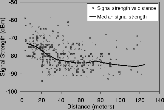
To characterize how observed 802.11 signal strengths varied with distance, we collected 500 readings at varying distances from a access points with well known locations in an urban area. Figure 1 illustrates the variation in signal strength for a single access point in a busy coffee shop as a function of the distance between the AP and the receiver. This graph plots the individual readings as well as showing how the median signal strength changes with distance.

The points for the individual readings show considerable spread for a given distance, and medium to weak readings (-70 to -90 dBm) occur at all distances. The curve showing the median signal strength does indicate however that there is a trend towards seeing weaker signals as distance from an access point grows. This indicates that while care needs to be taken, signal strength can be used as a weak indicator of distance and can thus be used to improve location estimation over simple observation.

Figure 2: Response rate for a single AP as a function of distance from that AP. Response rate is defined as follows: the percentage of times that a given AP was heard in all of the Wi-Fi scans at a specific distance from that AP. In the above graph we plot a histogram of response rate after grouping all distances into 5 meter buckets.

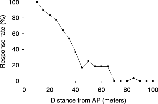In addition to signal strength, we explore a new metric for estimating a user's position. We define the response rate metric as follows: from the training data set, we collect all Wi-Fi scans that are at the same distance from an access point; we then compute the fraction of times that this AP is heard in that collection of Wi-Fi scans. For scans close to the AP, we expect the response rate to be high while for scans further away, with signal attenuation and interference, the AP is less likely to be heard and so the response rate will be low. We measured the response rate as a function of distance, and as can be seen in Figure 2, there is a strong correlation between the response rate and the distance from the AP. Our results may seem contradictory to the results from Roofnet [1], which shows packet loss rate has low correlation to distance. Roofnet measured the raw loss rate of 1500 byte broadcast packets across distant nodes (over 100 meters). On the other hand, we measure probe response rate of APs within 100 meters. The probe response packet is about 100 bytes and uses link-level unicast retransmissions. With shorter distance, smaller sized packets and link-level retransmissions, we noticed a stronger correlation between response rate and distance.

Figure 3: Variation in signal strength over a one hour period for three distinct access points measured at a single location.

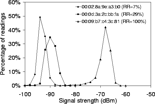These observations tend to reduce our confidence in algorithms that depend on signal strength varying predictably as a function of distance to the access point. Response rate appears to vary much more predictably vs. distance. However, even though the effect of distance is largely unpredictable, Figure 3 indicates that for a given location, signal strengths are relatively stable. Thus different locations may still be reliably identified by their signal strength signature. We test these beliefs experimentally in the remainder of this paper.

2 Positioning Algorithms

Based on the above observations, we looked at three classes of positioning algorithms. In this section, we present an overview of these algorithms.

1 Centroid

This is the simplest positioning algorithm. During the training phase, we combine all of the readings for a single access point and estimate a geographic location for the access point by computing the arithmetic mean of the positions reported in all of the readings. Thus, the radio map for this algorithm has one record per access point containing the estimated position of that AP.

Using this map, the centroid algorithm positions the user at the center of all of the APs heard during a scan by computing an average of the estimated positions of each of the heard APs. In addition to the simple arithmetic mean, we also experimented with a weighted version of this mechanism, where the position of each AP was weighted by the received signal strength during the scan.

2 Fingerprinting

This algorithm is based on an indoor positioning mechanism proposed in RADAR [2]. The hypothesis behind RADAR is as follows: at a given point, a user may hear different access points with certain signal strengths; this set of APs and their associated signal strengths represents a fingerprint that is unique to that position. As can be inferred from Figure 3, radio fingerprints are potentially a good indicator of a user's position. We used the same basic fingerprinting technique, but with the much coarser-grained war driving compared to the in-office dense dataset collected for RADAR. Thus, for fingerprinting, the radio map is the raw war-driving data itself, with each point in the map being a latitude-longitude coordinate and a fingerprint containing a scan of Wi-Fi access points and the signal strength with which they were heard.

In the positioning phase, a user's Wi-Fi device performs a scan of its environment. We compare this scan with all of the fingerprints in the radio map to find the fingerprint that is the closest match to the positioning scan in terms of APs seen and their corresponding signal strengths. The metric that we use for comparing various fingerprints is $k$-nearest-neighbor(s) in signal space as described in the original RADAR work. Suppose the positioning scan discovered three APs $A$, $B$, and $C$ with signal strengths $(SS_A, SS_B, SS_C)$. We determine the set of recorded fingerprints in the radio map that have the same set of APs and compute the distance in signal space between the observed signal strengths and the recorded ones in the fingerprints. Thus, for each matching fingerprint with signal strengths $(SS'_A, SS'_B, SS'_C)$, we compute the Euclidean distance:

$$\sqrt{(SS_A - SS'_A)^2 + (SS_B - SS'_B)^2 + (SS_C - SS'_C)^2}$$

To determine the user's position, we pick the $k$ fingerprints with the smallest distance to the observed scan and compute the average of the latitude-longitude coordinates associated with those $k$ fingerprints. Based on preliminary experiments with varying values of $k$, we discovered that $k=4$ provides good accuracy.

To account for APs that may have been deployed after the radio map was generated and for lost beacons from access points, we apply the following heuristics. First, during the positioning phase, if we discover any AP that never appears in the radio map, we ignore that AP. Second, when matching fingerprints to an observed scan, if we cannot find fingerprints with the same set of APs as heard in the scan, we expand the search to look for fingerprints that have supersets or subsets of the APs in the observed scan. We match fingerprints that have at most $p$ different APs between the fingerprint in the radio map and the observed scan. These heuristics help improve the matching rate for fingerprints significantly from 70% to 99%. Across all of our data sets, we found that $p=2$ provides the best matching rate without reducing overall accuracy.

Fingerprinting is based on the assumption that the Wi-Fi devices used for training and positioning measure signal strengths in the same way. If that is not the case (due to differences caused by manufacturing variations, antennas, orientation, etc.), one cannot directly compare the signal strengths. To account for this, we implemented a variation of fingerprinting called ranking inspired by an algorithm proposed for the RightSpot system [15]. Instead of comparing absolute signal strengths, this method compares lists of access points sorted by signal strength. For example, if the positioning scan discovered $(SS_A,SS_B,SS_C) = (-20, -90, -40)$, then we replace this set of signal strengths by their relative ranking, that is, $(R_A,R_B,R_C) = (1, 3, 2)$. Likewise, if $(SS'_A,SS'_B,SS'_C) = (-30, -15, -45)$, then $(R'_A,R'_B,R'_C) = (2,1,3)$. 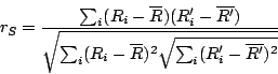We compare the relative rankings using the Spearman rank-order correlation coefficient [23]:

$$r_S = \frac {\sum_{i} (R_i - \overline{R})(R'_i - \overline{... ...- \overline{R})^2 \sqrt{ \sum_{i}(R'_i - \overline{R'})^2}}}$$

where $\overline{R}$ and $\overline{R'}$ are the means of the rank vectors. The Spearman coefficient ranges from $[-1,1]$, with higher values indicating more similar rankings. Using the relative order of signal strengths in this way means that fingerprints will still match well in spite of differences in scale, offset, or any monotonically increasing function of signal strength separating the Wi-Fi devices. To use ranking, the value of $r_S$ is substituted for the Euclidean distance in the fingerprint algorithm, and $r_S$ is negated to make more similar ranks give a smaller number.

3 Particle Filters

Particle filters have been used in the past, primarily in robotics, to past fuse a stream of sensor data into location estimates [9,21,13]. A particle filter is a probabilistic approximation algorithm that implements a Bayes filter [6]. It represents the location estimate of a user at time $t$ using a collection of weighted particles ${p^i_t, w^i_t}, (i = 1...n)$. Each $p^i_t$ is a distinct hypothesis about the user's current position. Each particle has a weight $w^i_t$ that represents the likelihood that this hypothesis is true, that is, the probability that the user's device would hear the observed scan if it were indeed at the position of the particle. A detailed description of the particle filter algorithm can be found in [13].

Particle-filter based location techniques require two input models: a sensor model and a motion model. The sensor model is responsible for computing how likely an individual particle's position is, given the observed sensor data. For Place Lab, the sensor model estimates how likely it is that a given set of APs would be observed at a given location. The motion model's job is to move the particles' locations in a manner that approximates the motion of the user.

For our experiments, we built two sensor models: one based on signal strength, while the other based on the response rate metric defined earlier. During the training phase, for each access point, we build an empirical model of how the signal strength and response rate vary by distance. Rather than fit the mapping data to a parametric function, Place Lab maintains a small table with an entry for each 5 meter increment in distance from the estimated AP location. Response rates are recorded as a percentage, while the signal strength distribution is recorded as a fraction of observations with low, medium and high strength for each distance bucket. The low/medium/high cut-offs are determined empirically to split the training data for each AP uniformly into the three categories. As an example, Place Lab will compute and record that for an AP $x$, its response rate at 60 meters is (say) 55%. We also record that at 60 meters, that AP will be seen with medium signal strength much more often than low or high. Given a new Wi-Fi scan, the sensor model determines a particle's likelihood as follows: for each AP in the scan, we look up the response rate or the probability of seeing the measured signal strength based on the distance between the particle and the estimated AP location in the radio map.

Place Lab uses a simple motion model that moves particles random distances in random directions. Our future work includes incorporation of more sophisticated motion models (such as those by Patterson et al. [22]) that model direction, velocity and even mode of transportation.

3 Data Collection

Figure 4: Density of access points (and satellite photos provided through Microsoft's Terraserver) for the neighborhoods in which we ran our experiments.

Table 1: AP density in the three areas measured per square kilometer and per Wi-Fi scan. The # APs/scan includes only those Wi-Fi scans that detected at least one access point.

Neighborhood	AP density	# APs/
	(APs/$km^2$)	scan
Downtown Seattle	1030	2.66
Ravenna	1000	2.56
Kirkland	130	1.41

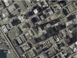
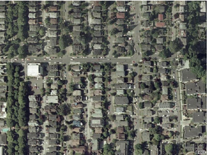
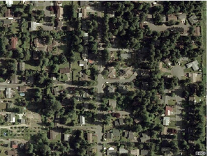
We collected traces of war-driving data in three neighborhoods in the Seattle metropolitan area:

• Downtown Seattle: a mix of commercial and residential urban high-rises
• Seattle's Ravenna neighborhood: a medium-density residential neighborhood
• Kirkland, Washington: a sparse suburb of single-family homes

For each neighborhood, we collected traces in two phases. First we constructed training data sets by driving around each neighborhood for thirty minutes with a Wi-Fi laptop and a GPS unit. Our data collection software performed Wi-Fi scans four times per second using an Orinoco-based 802.11b Wi-Fi card. GPS readings were logged approximately once per second. To assign latitude-longitude coordinates to each Wi-Fi scan, we used linear interpolation between consecutive GPS readings based on the timestamps associated with the Wi-Fi scans and the two GPS readings.

In the second phase, we collected another set of traces for each neighborhood. These traces are used as test data to estimate the positioning accuracy of the various Place Lab algorithms. In this phase, Place Lab used only the Wi-Fi scans collected in the trace, while the GPS readings were used as ``ground truth'' to compute the accuracy of the user's estimated position. To ensure that we gathered clean ground truth data, we tried to navigate within areas where the GPS device continuously reported a GPS lock and eliminated (and re-gathered) traces where the GPS data was obviously erroneous. Note that GPS has an accuracy of 5-7 meters, bounding the accuracy of our measurements to this level of granularity.

Even though Place Lab can be used both outdoors and indoors, most of our evaluation below is based on traces that were collected entirely outdoors. This limitation is due to the fact that we use GPS as ground truth and hence can evaluate Place Lab's performance only when GPS is available. In Section 4.6, we will present results from a simple experiment where we used Place Lab indoors.

4 Evaluation

In this section, we present our results from a suite of experiments conducted using the above data sets. Our results demonstrate the effect of varying a number of parameters on the accuracy of positioning using Place Lab.

1 Analysis of trace data

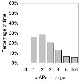
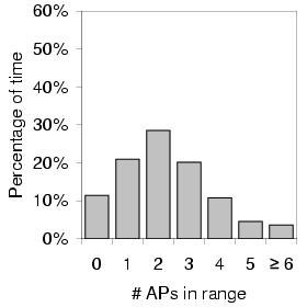
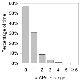
Figure 4 shows the distribution of the number of access points in range per scan for each of the three areas we measured. Table 1 shows the density of APs in the three areas. As expected, we noticed the highest density of APs in the downtown urban setting with an average of 2.66 APs per scan and no scans without APs. Also not surprisingly, the suburban traces saw zero APs (that is, no coverage) more than half the time and rarely saw more than one. Interestingly, the residential Ravenna data had almost the same number of APs per $km^2$ as downtown. With the exception of the approximately 10% of scans with no coverage, the AP density distribution for Ravenna fairly closely matched the downtown distribution.

Figure 5: CDF showing the median and maximum range of APs in meters.

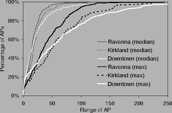
We also plotted the median and maximum range of each AP based on estimated positions of the AP from the radio map. Figure 5 shows a cumulative distribution function (CDF) of the median and maximum ranges for each of the three areas. In the relatively sparse Kirkland area, we notice that APs can be heard at a longer range than in Ravenna. We believe that this is due to the fact that Ravenna has a much denser distribution of access points and thus experiences higher interference (and consequently shorter range) as the data-gathering station gets further away from the AP. On the other hand, in downtown, which has about the same AP density as Ravenna, the maximum AP range is higher. This is due to the large number of tall buildings in downtown; APs that are located on higher floors often have a much longer range.

2 Relative performance

We now compare the relative performance of our positioning algorithms across the three areas. To evaluate the accuracy of Place Lab's positioning, we compare the position reported by Place Lab to that reported by the GPS device during the collection of the positioning trace. Table 2 summarizes the results. Ravenna, with its high density of short-range access points, performs the best and can estimate the user's position with a median error of 13-17 meters. Surprisingly, for Ravenna, there is little variation across the different algorithms. Even the simple centroid algorithms perform relatively well.

On the other hand, in Kirkland, with much lower AP density, we notice that the median positioning error is 2-3 times worse. But, as we move from the centroid algorithm to the particle-filter-based techniques, we notice a substantial improvement in accuracy (25% decrease in median error). In this case, the smarter algorithms were better able to filter through the sparse data and estimate the user's position. However, one algorithm that performed quite poorly in Kirkland is ranking. This is because of the significant number of times that a Wi-Fi scan produced a single AP. With just one AP, there can be no relative ranking, and hence the algorithm picks a random set of $k$ fingerprints that contain the AP and attempts to position the user at the average position of those randomly chosen fingerprints.

In the downtown area, even though the AP density is the same as Ravenna, median error is higher by 5-10 meters. This is due to the fact that APs in the tall buildings of downtown typically have a larger range and thus can be heard much further away than APs in Ravenna.

Table 2: Median error in meters for all of our algorithms across the three areas.

Algorithm		Downtown	Ravenna	Kirkland
		(meters)	(meters)	(meters)
centroid	basic	24.4	14.8	37.0
	weighted	23.4	14.5	37.0
fingerprint	radar	18.5	15.3	30.0
(k=4)	rank	20.3	16.7	59.5
particle filter	signal strength	18.0	14.4	29.7
	response rate	21.3	12.9	28.6

Figure 6: Median error as a function of number of APs heard in a scan (Kirkland).

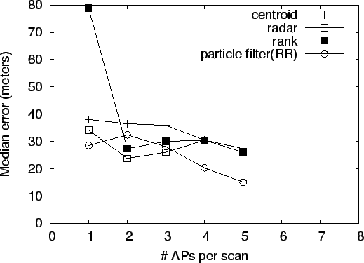
Finally, to understand the effect of the numbers of APs per scan on the positioning accuracy, we separated the output of the positioning traces based on the number of APs that were heard in each scan. For each group, we computed the median error. Figure 6 shows the median error as a function of the number of APs that were seen in a scan for one of the areas. Variants of algorithms that performed similar to their counterparts are left out for clarity. As we can see, the higher the number of APs heard during a scan, the lower the median positioning error. This graph also shows quite starkly the poor performance of ranking in the presence of a single known access point.

3 Effect of AP Turnover

Figure 7: Median error as a function of AP turnover (the percentage of APs that are deployed but are not part of the training data) for Ravenna. The coverage plot represents the variation in the percentage of time that at least one known AP was within range.

When building a metropolitan-scale positioning system, an important question to ask is how fresh the training data needs to be in order to produce reasonable positioning estimates. In particular, new access points may be deployed while existing APs are decommissioned. We can express AP turnover as the percentage of currently deployed access points that are not present in the training data set. To measure the effect of such obsolete training data, we generated variations of the three training sets (one for each area) by randomly dropping access points from the original data. This simulates the effect of having performed the training war drive before these APs were deployed. Note that decommissioned APs are, for the most part, less of a problem. They result in dead state in the training data and, except for fingerprinting, their presence in the training data does not affect the positioning algorithm.

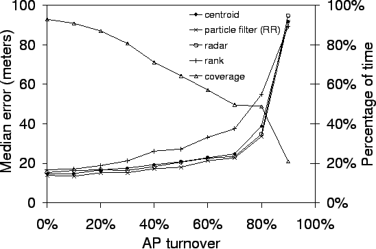
Figure 7 shows how AP turnover affects the median positioning error for the Ravenna neighborhood. From the figure, we can see that as the AP turnover rate increases, the coverage (that is, the percentage of time that at least one known AP is within range of the user) decreases. What is important to note though is that for most algorithms, an AP turnover of even 30% produces minimal effect on the positioning accuracy. The positioning error starts to increase noticeably only after at least half of the access points in the area have turned over. The exception to this is the ranking algorithm. Since it relies on a fairly coarse metric for positioning (relative rank order of AP signal strengths), the fewer APs available for this relative ordering, the worse its performance.

This data suggests that training data for an area does not need to be refreshed too often. Of course, the refresh rate (and exactly when to refresh) would depend on the turnover rate of APs in that area. Our experiments used variations that randomly dropped access points across the original training data. This is reasonable in dense urban areas as well as in residential neighborhoods where there are many uncorrelated deployments of access points. This is less true of large-scale deployments, say across a suburban office complex or a university campus, that span an entire neighborhood and are typically upgraded in lock step.

Correlated turnover can be an issue even in seemingly uncorrelated neighborhoods. As an anecdotal example, we looked at the AP turnover in the Ravenna neighborhood, which happens to be located near the University of Washington. Some of the blocks that we war drove are home to the university fraternity houses. We compared our Ravenna data set (which was gathered after the start of the school year) to another data set of the same neighborhood that we gathered earlier during the middle of the summer. At least 50% of the APs in the later set of traces did not appear in our earlier traces. This was due to the fact that between our two experiments, new students had arrived for the fall quarter while summer students left en masse. Hence, when determining the schedule and frequency of refresh for the training data, it is important to take into account such social factors that can have a significant effect on the deployment of access points.

4 Effect of noisy GPS data

Figure 8: Median positioning error as a function of the standard deviation of GPS noise (Ravenna).

Figure 9: Median positioning error as a function of the standard deviation of GPS noise (Downtown).

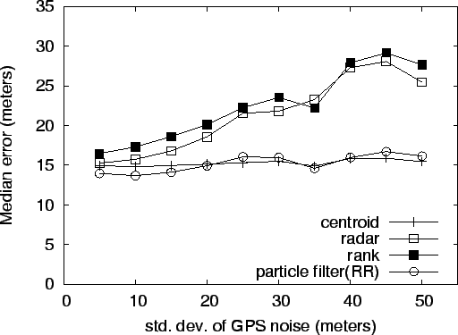
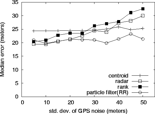
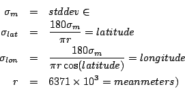
Some geographic regions will have higher GPS errors than others, due to urban canyons or foliage. This next experiment was designed to measure how robust the algorithms are to errors in the measured positions of the training data, which are normally measured via GPS. One way to assess the effect of poor GPS data would be to single out those areas where the GPS data is known to be poor. However, such locations may well exhibit Wi-Fi anomalies like multipath in urban canyons or RF blockage in areas of thick foliage [19]. In order to assess the overall effect of inaccurate GPS data on all our test data, we added zero mean Gaussian noise to the originally measured latitude-longitude readings in the training data. To make the results easier to understand, we specified the standard deviation of the noise in meters and converted to degrees latitude or longitude with the following:

$$\begin{eqnarray*} \sigma_m & = & stddev\in\meters \\ \sigma_{lat} & = & \frac... ...stddev\\ r & = & 6371 \times 10^3 = mean\earth\radius\(meters) \end{eqnarray*}$$

We used these modified training data sets to generate new radio maps and then computed the positioning error by running the unmodified test traces through these maps. Figure 8 shows the effect that GPS noise has on positioning accuracy. For the centroid algorithms, with sufficient number of observations, the GPS noise cancels out while creating the radio map. Hence we see no discernible effect on the performance of the centroid algorithm. Similarly, the particle filter techniques rely on empirical models built using the same radio map. Some error is introduced into these models because each of the readings that contribute to the histogram for the model has noisy positioning data, and thus can get misclassified. However the effect of this is not substantial as seen in Figure 8. On the other hand, for the fingerprinting techniques, the raw (and noisy) GPS positions are used directly in the radio map. Hence these techniques suffer the most in the presence of GPS noise. Figure 9 shows the same experiment for the Downtown data set. Similar trends are visible in this graph, as well as for the Kirkland data (not shown).

5 Density of mapping data

In the next experiment, we vary the geometric density of mapping points in the training data set. We expect the accuracy will go down with decreasing density of training data points. This variation is intended to find the effect of reduced density in the training set (which in turn means less calibration). We measured training density as the mean distance from each point (latitude-longitude coordinate) in the training data set to its geometrically nearest neighbor. In order to generate this variation, we first split the training file into a grid of 10m $\times$ 10m cells. We then eliminated Wi-Fi scans from the training data set one by one, creating a new mapping file after each elimination. To pick the next point to eliminate, we randomly picked one point in the cell with the highest population of points. If two or more cells tied for the maximum number of points, we picked between those tied cells at random. By eliminating points from the cells with the highest population, this algorithm tended to eliminate points around higher densities, driving the training files toward a more uniform density of data points for testing.

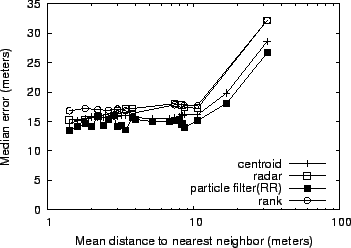
Figure 10 shows the median positioning error as a function of the average distance to the nearest neighbor in the training data set. The higher the average distance, the sparser the data set. From the figure, we can see that until the mapping density drops below 10 meter average distance between points, there is no appreciable effect on median error. Beyond that point, however, the positioning error increases sharply. There is not much distinction in this behavior across the various algorithms. This suggests that a training map generated at a scanning rate of one Wi-Fi scan per second and a driving speed of 20-25 miles/hour (or faster speeds with repeated drives through the same neighborhood) is sufficient to provide reasonable accuracy.

Figure 10: Positioning error as a function of the average distance between points in the training data set (Ravenna). Note that the x-axis is a logarithmic scale.

6 An Indoor Usage Scenario

All of the above experiments used training and positioning data sets that were collected entirely outdoors. Since the training data requires GPS, it must necessarily be collected outdoors. In the positioning phase, Place Lab can be used both outdoors and indoors. However, it is difficult to quantify the accuracy while indoors since we cannot collect any ground truth GPS data. To demonstrate the usability of Place Lab indoors, we ran a simple experiment where we collected two-minute-long positioning traces in nine different indoor locations, along with longer outdoor training traces around those locations. For each location, we computed the average position estimated by Place Lab. In addition, we determined average latitude-longitude positions for all nine locations by plotting their addresses into a mapping tool (MapPoint). Table 3 summarizes the error between Place Lab's average estimate and the latitude-longitude position from MapPoint.

The average error from this simple experiment ranges from 9 to 98 meters. Although at the high end the average error is significantly higher than in our previous experiments, it comes partially from inaccurate ground truth data: we used a single latitude-longitude point to represent each location when in fact each building may be several tens of meters across. We stress that this experiment is not an attempt to draw general conclusions about the accuracy of Place Lab when used indoors with training data that was collected outdoors. The experiment only serves to show that unlike GPS, Place Lab works indoors (and when there is no line of sight to the sky). Of course, one should remember that the limited calibration associated with Place Lab inherently means that it cannot be used for precise indoor location applications.

Table 3: Average error with Place Lab when used in indoor settings.

Location	Avg. error
	(meters)
Home 1	9.0
CS department	9.1
Downtown mall	9.5
Office	34.2
Bakery	38.9
Home 2	84.3
Doctor's office	85.2
Café	92.4
Home 3	98.7

7 Summary of Results

To summarize the results from the above experiments, we noted a few dominant effects that play a role in positioning accuracy using the various location techniques.

• The density of access points as well as the average range of APs in a region affect the positioning accuracy. In our experiments, we discovered that the Ravenna neighborhood with a dense collection of APs in low-rise buildings provided the best accuracy while suburban neighborhoods with sparse coverage showed the least accuracy.

• In dense urban environments, even a simple centroid-based positioning algorithm provides the same accuracy as more complex techniques. The complex techniques are more valuable in sparser environments with limited calibration data.

• Even a radio map that is old enough to have only 50% of the deployed APs is sufficient without degrading positioning accuracy by more than a few meters. Our mapping density experiments show that training data collected at the rate of one scan per second with a driving speed of 20-25 miles/hour is enough to build accurate radio maps.

• Noise in GPS data (which can result from either poor GPS units or due to urban canyons) affects fingerprint-based techniques much more than the other techniques. Thus, in environments where it is hard to collect accurate GPS data for training, we expect the particle-filter-based algorithms to perform better.

• The rank fingerprint algorithm was usually among the worst performing algorithms. Its poor performance was largely due to the fact that it throws away absolute signal strengths. However, in return, it also sheds its sensitivity to potential systematic differences in the way different Wi-Fi devices measure signal strength.

5 Discussion

We now discuss some of the practical issues that must be addressed when deploying such a system in the real world. Our experimental setup used active scanning to probe for nearby access points. However, APs can sometimes be configured to not respond to broadcast probe packets. Moreover, they may never send out broadcast beacon packets announcing their presence either. In such scenarios, passive scanning where the Wi-Fi card does not send out probe requests, and instead simply sniffs traffic on each of the Wi-Fi channels, may be used. Passive scanning relies on network traffic to discover APs and hence can detect even cloaked APs that do not necessarily advertise their network IDs.

All of our experiments were performed in outdoor environments since we needed access to GPS data even for our positioning traces to allow us to compare Place Lab's estimated positions to some known ground truth. However, Place Lab can work indoors as well. Even though we were unable to perform extensive experiments to measure Place Lab's accuracy when indoors, our regular use of Place Lab in a variety of indoor situations has shown that it can routinely position the user within less than one city block of their true position. As long as the user's device can hear access points that have been mapped out, Place Lab can estimate its position. This accuracy is not sufficient for indoor location applications that require room-level (or greater) accuracy, but is more than enough for other coarser-grained applications. For such applications, Place Lab can function as a GPS replacement that works both indoors and outdoors.

We used Wi-Fi cards based on the Orinoco chipset for all of our experiments. As pointed out in [10], different chipsets can report different signal strength values for the same AP at the same location. This is because each chipset interprets the raw signal strength value differently. However, there is a linear correlation for measured signal strengths across chipsets. This was first shown by Haeberlen et. al. [10]. We validated this claim for the following chipsets: Orinoco, Prism 2, Aironet, and Atheros. If we record the chipset information when collecting data sets, then even if the positioning is done using a chipset that is different from the one used for collecting the training data, a simple linear transformation will be sufficient to map the signal strength values across them. Of course, this is important only for those algorithms that actually rely on signal strength for positioning.

As the first systematic study of metropolitan-scale Wi-Fi localization, our accuracy comparisons suggest what to pursue in terms of new positioning algorithms. We found that different algorithms work best with different densities and ranges of access points. Since both of these quantities can be measured beforehand, the best algorithm could be automatically switched in depending on the current situation. Further, the size of the radio map can be a substantial issue for small mobile devices. The centroid and particle filter radio maps are relatively compact whereas fingerprinting algorithms require the entire training data set as their radio map. If (say for privacy concerns), the user wishes to store the radio map for their region on their local device, this may be a factor in determining the appropriate algorithm to use.

Our studies also compare the effects of density of calibration data, noise in calibration, and age of data on the centroid, particle filter and fingerprinting algorithms. An algorithm combining these techniques is feasible, and it may prove to be both robust and accurate. Moreover, one could incorporate additional environmental data such as (for example) constrained GIS maps of city streets and highways for navigation applications to improve the positioning accuracy. While we leave these ideas for future work, our study gives a concrete basis for choosing what to do next.

6 Conclusion

Place Lab is an attempt at providing ubiquitous Wi-Fi-based positioning in metropolitan areas. In this paper, we compared a number of Wi-Fi positioning algorithms in a variety of scenarios. Our results show that in dense urban areas Place Lab's positioning accuracy is between 13-20 meters. In more suburban neighborhoods, accuracy can drop down to 40 meters. Moreover, with dense Wi-Fi coverage, the specific algorithm used for positioning is not as important as other factors including composition of the neighborhood (lots of tall buildings versus low-rises), age of training data, density of training data sets, and noise in the training data. In sparser neighborhoods, sophisticated algorithms that can model the environment more richly win out. All of this positioning accuracy (although lower than that provided by precise indoor positioning systems) can be achieved with substantially less calibration effort: half an hour to map out an entire city neighborhood as compared to over 10 hours for a single office building [10].

Interested readers may download the data sets used for these experiments and the Place Lab source code from http://www.placelab.org/.

7 References

1

D. Aguayo, J. Bicket, S. Biswas, G. Judd, and R. Morris.
Link-level measurements from an 802.11b mesh network.
In Proceedings of SIGCOMM '04, Aug. 2004.

2

P. Bahl and V. N. Padmanabhan.
RADAR: An In-Building RF-Based User Location and Tracking System.
In Proceedings of IEEE Infocom 00, April 2000.

3

Dodgeball.com.
Mobile social software.
http://www.dodgeball.com/.

4

E911 and E112 Resources.
http://www.globallocate.com/.

5

P. Enge and P. Misra.
The Global Positioning System.
Proceedings of the IEEE (Special Issue on GPS), pages 3-172, January 1999.

6

D. Fox, J. Hightower, L. Liao, D. Schulz, and G. Borriello.
Bayesian filtering for location estimation.
IEEE Pervasive Computing, 2(3):24-33, July-September 2003.

7

Google.com.
Google local: Find local businesses and services on the web.
http://local.google.com/.

8

B. G. Griswold et al.
Using mobile technology to create opportunistic interaction on a university campus.
In Proceedings of UBICOMP Workshop on Supporting Spontaneous Interaction in Ubiquitous Computing Settings, September 2002.

9

F. Gustafsson, F. Gunnarsson, N. Bergman, U. Forssell, J. Jansson, R. Karlsson, and P.-J. Nordlund.
Particle Filters for Positioning, Navigation and Tracking.
IEEE Transactions on Signal Processing, 50:425-435, February 2002.

10

A. Haeberlen, E. Flannery, A. M. Ladd, A. Rudys, D. S. Wallach, and L. E. Kavraki.
Practical robust localization over large-scale 802.11 wireless networks.
In Proceedings of ACM MobiCom, Philadelphia, PA, Sept. 2004.

11

J. Hightower and G. Borriello.
Location systems for ubiquitous computing.
IEEE Computer, 34(8):57-66, August 2001.

12

J. Hightower and G. Borriello.
Accurate, Flexible, and Practical Location Estimation for Ubiquitous Computing.
In Proceedings of International Conference on Ubiquitous Computing (UBICOMP), 2004.

13

J. Hightower and G. Borriello.
Particle filters for location estimation in ubiquitous computing: A case study.
In Proceedings of International Conference on Ubiquitous Computing (UBICOMP), 2004.

14

Kismet.
http://www.kismetwireless.net/.

15

J. Krumm, G. Cermak, and E. Horvitz.
RightSPOT: A Novel Sense of Location for a Smart Personal Object.
In Proceedings of International Conference on Ubiquitous Computing (UBICOMP), October 2003.

16

J. Krumm and E. Horvitz.
Locadio: Inferring motion and location from wi-fi signal strengths.
In Proceedings of International Conference on Mobile and Ubiquitous Systems: Networking and Services (MobiQuitous'04), 2004.

17

A. M. Ladd, K. E. Bekris, A. Rudys, G. Marceau, and L. E. Kavraki.
Robotics-Based Location Sensing Using Wireless Ethernet.
In Proceedings of ACM MobiCom, September 2002.

18

A. LaMarca et al.
Place lab: Device positioning using radio beacons in the wild.
In Proceedings of International Conference on Pervasive Computing (Pervasive), June 2005.

19

C. Ma, G.-I. Jee, G. MacGougan, G. Lachapelle, S. Bloebaum, G. Cox, L. Garin, and J. Shewfelt.
Gps signal degradation modeling.
In Proceedings of International Technical Meeting of the Satellite Division of the Institute of Navigation, Sept. 2001.

20

NetStumbler.
http://www.netstumbler.com.

21

P.-J. Norlund, F. Gunnarsson, and F. Gustafsson.
Particle Filters for Positioning in Wireless Networks.
In Proceedings of EUSIPCO, September 2002.

22

D. J. Patterson, L. Liao, D. Fox, and H. Kautz.
Inferring High-Level Behavior from Low-Level Sensors.
In Proceedings of International Conference on Ubiquitous Computing (UBICOMP), 2003.

23

W. H. Press, S. A. Teukolsky, W. T. Vetterling, and B. P. Flannery.
Numerical Recipes in C.
Cambridge University Press, 1992.

24

N. B. Priyantha, A. Chakraborty, and H. Balakrishnan.
The Cricket Location-Support System.
In Proceedings of ACM MobiCom'00, July 2000.

25

M. Rabinowitz and J. Spilker.
A new positioning system using television synchronization signals.
http://www.rosum.com/.

26

T. Roos, P. Myllymaki, H. Tirri, P. Misikangas, and J. Sievanan.
A probabilistic approach to wlan user location estimation.
International Journal of Wireless Information Networks, 9(3), July 2002.

27

B. N. Schilit, N. Adams, R. Gold, M. Tso, and R. Want.
The PARCTAB Mobile Computing System.
In Proceedings of Workshop on Workstation Operating Systems, pages 34-39, Oct. 1993.

28

I. Smith et al.
Social disclosure of place: From location technology to communication practices.
In Proceedings of International Conference on Pervasive Computing (Pervasive), May 2005.

29

R. Want, A. Hopper, V. Falcao, and J. Gibbons.
The Active Badge Location System.
ACM Transactions on Information Systems, 1992.

30

Yahoo! Inc.
Yahoo local: Find businesses and services near you.
http://local.yahoo.com/.

Footnoots

... data.

Dodgeball.com, for example, hosts a cellphone-based social meet-up application with thousands of daily users and relies on zipcodes to represent users' locations. It is well within Place Lab's ability to accurately estimate zip code.

... points.

Instead of active scanning, one could use passive scanning by listening on each Wi-Fi channel for beacon frames from the nearby access points.

... shop

We observed similar behavior from the other access points and we show one AP's data for the sake of clarity.

... mean

We do not in fact compute the centroid, but we still name this method as such instead of using the term ``mean'' so as to disambiguate the heuristic from other uses of arithmetic mean during the discussion of our experimental results.

... area

Although the Seattle metropolitan area is a tech-friendly environment and consequently has a higher proliferation of Wi-Fi access points than many other parts of the country (or the world), we believe that it represents the leading edge of an upward growth trend. So although results from these areas may not necessarily apply today to other cities with lower Wi-Fi coverage, we expect other metro areas will eventually match Seattle's current coverage density.

... neighborhood.

Other neighborhoods showed similar behavior and their data is left out for clarity

... set.

Note that some of the highest density data points in the graph arise as a result of the fact that we sometimes war drove the same streets more than once thus generating a denser training data set.

... miles/hour

10 meters between scans is equivalent to a driving speed of $10 \times 3600$ meters/hour, that is, 22.5 miles/hour.

MobiSys '05 Technical Program MobiSys '05 Home USENIX home